The ANSS event ID is usp000e2bp and the event page is at https://earthquake.usgs.gov/earthquakes/eventpage/usp000e2bp/executive.
2005/10/20 21:16:28 44.677 -80.482 11.0 4.2 Quebec, Canada
 USGS/SLU Moment Tensor Solution
 ENS  2005/10/20 21:16:28:0  44.68  -80.48  11.0 4.2 Quebec, Canada

 Stations used:
   CN.ALGO CN.BANO CN.BRCO CN.BUKO CN.DELO CN.ELFO CN.GAC
   CN.KAPO CN.KGNO CN.MEDO CN.MNT CN.PECO CN.PKRO CN.PLIO
   CN.RSPO CN.SADO

 Filtering commands used:
   cut o DIST/3.3 -40 o DIST/3.3 +50
   rtr
   taper w 0.1
   hp c 0.03 n 3
   lp c 0.10 n 3
   br c 0.12 0.25 n 4 p 2

 Best Fitting Double Couple
  Mo = 3.27e+21 dyne-cm
  Mw = 3.61
  Z  = 10 km
  Plane   Strike  Dip  Rake
   NP1      167    67    99
   NP2      325    25    70
  Principal Axes:
   Axis    Value   Plunge  Azimuth
    T   3.27e+21     67      94
    N   0.00e+00      8     343
    P  -3.27e+21     21     250

 Moment Tensor: (dyne-cm)
    Component   Value
       Mxx    -3.31e+20
       Mxy    -9.45e+20
       Mxz     3.03e+20
       Myy    -2.03e+21
       Myz     2.20e+21
       Mzz     2.36e+21


                     ##------------
                 #----#######----------
              --------############--------
             --------###############-------
           ----------#################-------
          -----------###################------
         ------------####################------
        -------------#####################------
        -------------######################-----
       --------------#######################-----
       ---------------##########   #########-----
       ---------------########## T ##########----
       ----------------#########   ##########----
        ---   ---------######################---
        --- P ----------#####################---
         --   ----------####################---
          ---------------###################--
           ---------------#################--
             --------------###############-
              --------------#############-
                 -------------#########
                     -----------###


 Global CMT Convention Moment Tensor:
      R          T          P
  2.36e+21   3.03e+20  -2.20e+21
  3.03e+20  -3.31e+20   9.45e+20
 -2.20e+21   9.45e+20  -2.03e+21


Details of the solution is found at

http://www.eas.slu.edu/eqc/eqc_mt/MECH.NA/20051020211628/index.html
|
      STK = 325
      DIP = 25
     RAKE = 70
       MW = 3.61
       HS = 10.0
The NDK file is 20051020211628.ndk The waveform inversion is preferred.
|
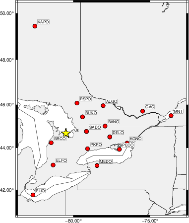
The focal mechanism was determined using broadband seismic waveforms. The location of the event (star) and the stations used for (red) the waveform inversion are shown in the next figure.
|
|
|
The program wvfgrd96 was used with good traces observed at short distance to determine the focal mechanism, depth and seismic moment. This technique requires a high quality signal and well determined velocity model for the Green's functions. To the extent that these are the quality data, this type of mechanism should be preferred over the radiation pattern technique which requires the separate step of defining the pressure and tension quadrants and the correct strike.
The observed and predicted traces are filtered using the following gsac commands:
cut o DIST/3.3 -40 o DIST/3.3 +50
rtr
taper w 0.1
hp c 0.03 n 3
lp c 0.10 n 3
br c 0.12 0.25 n 4 p 2
The results of this grid search are as follow:
           DEPTH  STK   DIP  RAKE   MW    FIT
WVFGRD96    1.0   165    45    85   3.47 0.5069
WVFGRD96    2.0   160    50    80   3.55 0.4507
WVFGRD96    3.0   350    90   -80   3.59 0.4894
WVFGRD96    4.0   175    80    75   3.59 0.5693
WVFGRD96    5.0   175    75    75   3.60 0.6226
WVFGRD96    6.0   325    20    70   3.60 0.6618
WVFGRD96    7.0   330    25    75   3.62 0.6871
WVFGRD96    8.0   325    25    70   3.60 0.7016
WVFGRD96    9.0   320    30    65   3.61 0.7065
WVFGRD96   10.0   325    25    70   3.61 0.7071
WVFGRD96   11.0   320    30    65   3.62 0.7050
WVFGRD96   12.0   320    30    65   3.62 0.7002
WVFGRD96   13.0   320    30    60   3.62 0.6947
WVFGRD96   14.0   315    30    55   3.61 0.6876
WVFGRD96   15.0   315    30    55   3.61 0.6799
WVFGRD96   16.0   315    30    55   3.62 0.6709
WVFGRD96   17.0   315    30    55   3.62 0.6608
WVFGRD96   18.0   310    30    50   3.62 0.6498
WVFGRD96   19.0   310    30    50   3.63 0.6376
WVFGRD96   20.0   310    30    50   3.66 0.6265
WVFGRD96   21.0   310    30    50   3.67 0.6111
WVFGRD96   22.0   305    30    45   3.68 0.5944
WVFGRD96   23.0   305    30    45   3.68 0.5761
WVFGRD96   24.0   310    25    50   3.68 0.5565
WVFGRD96   25.0   310    25    50   3.69 0.5357
WVFGRD96   26.0   155    65    55   3.73 0.5151
WVFGRD96   27.0   215    55   -40   3.78 0.5034
WVFGRD96   28.0   215    55   -35   3.79 0.4893
WVFGRD96   29.0   215    55   -35   3.80 0.4755
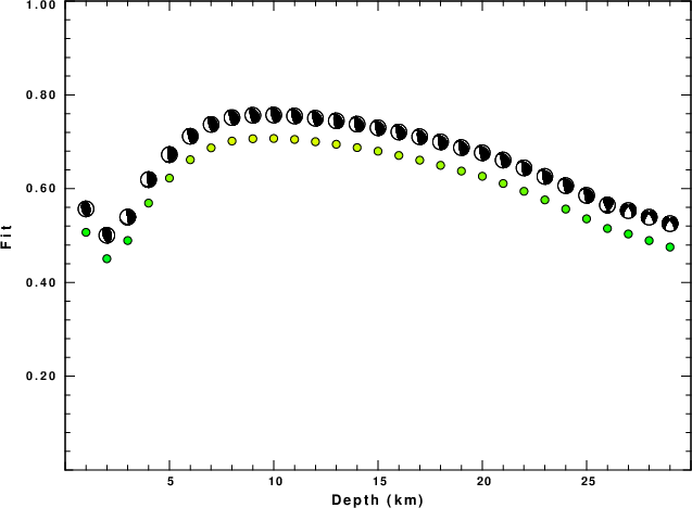
The best solution is
WVFGRD96 10.0 325 25 70 3.61 0.7071
The mechanism corresponding to the best fit is
|
|
|
The best fit as a function of depth is given in the following figure:
|
|
|
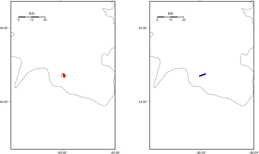
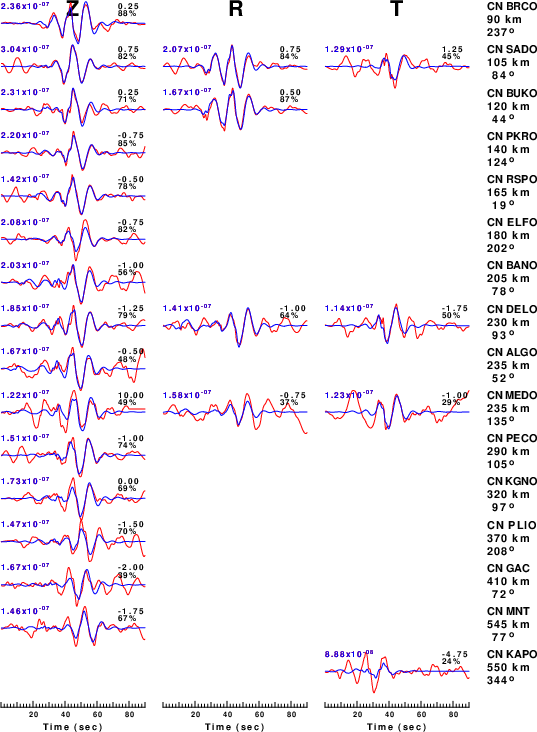
The comparison of the observed and predicted waveforms is given in the next figure. The red traces are the observed and the blue are the predicted. Each observed-predicted component is plotted to the same scale and peak amplitudes are indicated by the numbers to the left of each trace. A pair of numbers is given in black at the right of each predicted traces. The upper number it the time shift required for maximum correlation between the observed and predicted traces. This time shift is required because the synthetics are not computed at exactly the same distance as the observed, the velocity model used in the predictions may not be perfect and the epicentral parameters may be be off. A positive time shift indicates that the prediction is too fast and should be delayed to match the observed trace (shift to the right in this figure). A negative value indicates that the prediction is too slow. The lower number gives the percentage of variance reduction to characterize the individual goodness of fit (100% indicates a perfect fit).
The bandpass filter used in the processing and for the display was
cut o DIST/3.3 -40 o DIST/3.3 +50
rtr
taper w 0.1
hp c 0.03 n 3
lp c 0.10 n 3
br c 0.12 0.25 n 4 p 2
|
| Figure 3. Waveform comparison for selected depth. Red: observed; Blue - predicted. The time shift with respect to the model prediction is indicated. The percent of fit is also indicated. The time scale is relative to the first trace sample. |
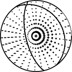
|
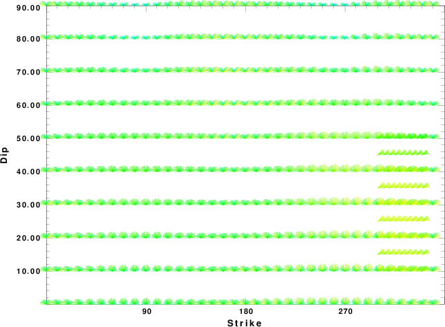
| Focal mechanism sensitivity at the preferred depth. The red color indicates a very good fit to the waveforms. Each solution is plotted as a vector at a given value of strike and dip with the angle of the vector representing the rake angle, measured, with respect to the upward vertical (N) in the figure. |
A check on the assumed source location is possible by looking at the time shifts between the observed and predicted traces. The time shifts for waveform matching arise for several reasons:
Time_shift = A + B cos Azimuth + C Sin Azimuth
The time shifts for this inversion lead to the next figure:
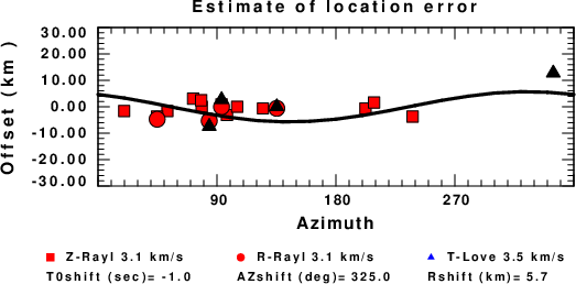
The derived shift in origin time and epicentral coordinates are given at the bottom of the figure.
The CUS.model used for the waveform synthetic seismograms and for the surface wave eigenfunctions and dispersion is as follows (The format is in the model96 format of Computer Programs in Seismology).
MODEL.01
CUS Model with Q from simple gamma values
ISOTROPIC
KGS
FLAT EARTH
1-D
CONSTANT VELOCITY
LINE08
LINE09
LINE10
LINE11
  H(KM) VP(KM/S) VS(KM/S) RHO(GM/CC)   QP   QS  ETAP  ETAS  FREFP  FREFS
  1.0000  5.0000  2.8900  2.5000 0.172E-02 0.387E-02 0.00  0.00  1.00  1.00
  9.0000  6.1000  3.5200  2.7300 0.160E-02 0.363E-02 0.00  0.00  1.00  1.00
 10.0000  6.4000  3.7000  2.8200 0.149E-02 0.336E-02 0.00  0.00  1.00  1.00
 20.0000  6.7000  3.8700  2.9020 0.000E-04 0.000E-04 0.00  0.00  1.00  1.00
  0.0000  8.1500  4.7000  3.3640 0.194E-02 0.431E-02 0.00  0.00  1.00  1.00