Location
Location ANSS
The ANSS event ID is usp000cz1k and the event page is at
https://earthquake.usgs.gov/earthquakes/eventpage/usp000cz1k/executive.
2004/06/28 06:10:52 41.460 -88.900 10.0 4.2 Illinois
Focal Mechanism
 USGS/SLU Moment Tensor Solution
 ENS  2004/06/28 06:10:52:0  41.46  -88.90  10.0 4.2 Illinois

 Stations used:
   _.BLO _.CCM _.FVM _.JFWS _.SLM
   _.USIN _.WCI PN.PPFAY PN.PPMSH PN.PPNAF PN.PPNVW

 Filtering commands used:
   cut o DIST/3.3 -40 o DIST/3.3 +50
   rtr
   taper w 0.1
   hp c 0.03 n 3
   lp c 0.10 n 3

 Best Fitting Double Couple
  Mo = 1.17e+22 dyne-cm
  Mw = 3.98
  Z  = 8 km
  Plane   Strike  Dip  Rake
   NP1      199    85   170
   NP2      290    80     5
  Principal Axes:
   Axis    Value   Plunge  Azimuth
    T   1.17e+22     11     154
    N   0.00e+00     79     353
    P  -1.17e+22      4     245

 Moment Tensor: (dyne-cm)
    Component   Value
       Mxx     7.10e+21
       Mxy    -8.94e+21
       Mxz    -1.60e+21
       Myy    -7.45e+21
       Myz     1.58e+21
       Mzz     3.50e+20


                     ##############
                 #################-----
              ###################---------
             ###################-----------
           ####################--------------
          ####################----------------
         #####################-----------------
        ------###############-------------------
        --------------######--------------------
       ------------------------------------------
       --------------------######----------------
       -------------------###########------------
       -------------------###############--------
        -----------------###################----
           --------------######################-
         P -------------#######################
           ------------#######################
           ------------######################
             ---------#####################
              --------#############   ####
                 -----############# T #
                     ##############


 Global CMT Convention Moment Tensor:
      R          T          P
  3.50e+20  -1.60e+21  -1.58e+21
 -1.60e+21   7.10e+21   8.94e+21
 -1.58e+21   8.94e+21  -7.45e+21


Details of the solution is found at

http://www.eas.slu.edu/eqc/eqc_mt/MECH.NA/20040628061052/index.html
|
Preferred Solution
The preferred solution from an analysis of the surface-wave spectral amplitude radiation pattern, waveform inversion or first motion observations is
      STK = 290
      DIP = 80
     RAKE = 5
       MW = 3.98
       HS = 8.0
The NDK file is 20040628061052.ndk
The waveform inversion is preferred.
Moment Tensor Comparison
The following compares this source inversion to those provided by others. The purpose is to look for major differences and also to note slight differences that might be inherent to the processing procedure. For completeness the USGS/SLU solution is repeated from above.
| SLU |
LDEO |
 USGS/SLU Moment Tensor Solution
 ENS  2004/06/28 06:10:52:0  41.46  -88.90  10.0 4.2 Illinois

 Stations used:
   _.BLO _.CCM _.FVM _.JFWS _.SLM
   _.USIN _.WCI PN.PPFAY PN.PPMSH PN.PPNAF PN.PPNVW

 Filtering commands used:
   cut o DIST/3.3 -40 o DIST/3.3 +50
   rtr
   taper w 0.1
   hp c 0.03 n 3
   lp c 0.10 n 3

 Best Fitting Double Couple
  Mo = 1.17e+22 dyne-cm
  Mw = 3.98
  Z  = 8 km
  Plane   Strike  Dip  Rake
   NP1      199    85   170
   NP2      290    80     5
  Principal Axes:
   Axis    Value   Plunge  Azimuth
    T   1.17e+22     11     154
    N   0.00e+00     79     353
    P  -1.17e+22      4     245

 Moment Tensor: (dyne-cm)
    Component   Value
       Mxx     7.10e+21
       Mxy    -8.94e+21
       Mxz    -1.60e+21
       Myy    -7.45e+21
       Myz     1.58e+21
       Mzz     3.50e+20


                     ##############
                 #################-----
              ###################---------
             ###################-----------
           ####################--------------
          ####################----------------
         #####################-----------------
        ------###############-------------------
        --------------######--------------------
       ------------------------------------------
       --------------------######----------------
       -------------------###########------------
       -------------------###############--------
        -----------------###################----
           --------------######################-
         P -------------#######################
           ------------#######################
           ------------######################
             ---------#####################
              --------#############   ####
                 -----############# T #
                     ##############


 Global CMT Convention Moment Tensor:
      R          T          P
  3.50e+20  -1.60e+21  -1.58e+21
 -1.60e+21   7.10e+21   8.94e+21
 -1.58e+21   8.94e+21  -7.45e+21


Details of the solution is found at

http://www.eas.slu.edu/eqc/eqc_mt/MECH.NA/20040628061052/index.html
|
Solution by Won-Young Kim
at Lamont-Doherty Earth Observatory of Columbia University
|
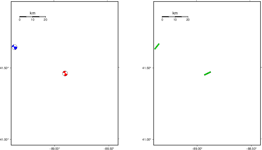
Context
The left panel of the next figure presents the focal mechanism for this earthquake (red) in the context of other nearby events (blue) in the SLU Moment Tensor Catalog. The right panel shows the inferred direction of maximum compressive stress and the type of faulting (green is strike-slip, red is normal, blue is thrust; oblique is shown by a combination of colors). Thus context plot is useful for assessing the appropriateness of the moment tensor of this event.
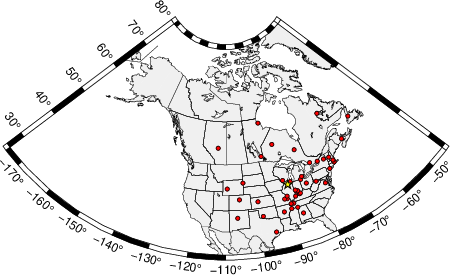
Waveform Inversion using wvfgrd96
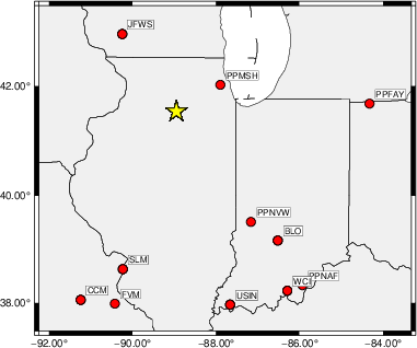
The focal mechanism was determined using broadband seismic waveforms. The location of the event (star) and the
stations used for (red) the waveform inversion are shown in the next figure.
|
|
Location of broadband stations used for waveform inversion
|
The program wvfgrd96 was used with good traces observed at short distance to determine the focal mechanism, depth and seismic moment. This technique requires a high quality signal and well determined velocity model for the Green's functions. To the extent that these are the quality data, this type of mechanism should be preferred over the radiation pattern technique which requires the separate step of defining the pressure and tension quadrants and the correct strike.
The observed and predicted traces are filtered using the following gsac commands:
cut o DIST/3.3 -40 o DIST/3.3 +50
rtr
taper w 0.1
hp c 0.03 n 3
lp c 0.10 n 3
The results of this grid search are as follow:
           DEPTH  STK   DIP  RAKE   MW    FIT
WVFGRD96    1.0   290    70   -20   3.76 0.4654
WVFGRD96    2.0   290    85     5   3.82 0.5300
WVFGRD96    3.0   290    80    15   3.89 0.5685
WVFGRD96    4.0   290    80    15   3.93 0.5782
WVFGRD96    5.0   290    70     5   3.94 0.5905
WVFGRD96    6.0   290    75     5   3.96 0.6337
WVFGRD96    7.0   290    75     5   3.97 0.6560
WVFGRD96    8.0   290    80     5   3.98 0.6622
WVFGRD96    9.0   290    80     5   3.99 0.6603
WVFGRD96   10.0   290    80     5   4.00 0.6516
WVFGRD96   11.0   290    80     5   4.00 0.6328
WVFGRD96   12.0   290    80     5   4.00 0.6095
WVFGRD96   13.0   290    80     5   4.01 0.5852
WVFGRD96   14.0   290    85     5   4.01 0.5621
WVFGRD96   15.0   290    85     5   4.02 0.5397
WVFGRD96   16.0   110    90     0   4.03 0.5214
WVFGRD96   17.0   110    90     0   4.03 0.5033
WVFGRD96   18.0   110    90     0   4.04 0.4843
WVFGRD96   19.0   110    90     0   4.05 0.4669
WVFGRD96   20.0   110    90     0   4.07 0.4491
WVFGRD96   21.0   290    90     0   4.07 0.4297
WVFGRD96   22.0   110    90     0   4.07 0.4107
WVFGRD96   23.0   115    90     0   4.07 0.3922
WVFGRD96   24.0   115    90     0   4.08 0.3742
WVFGRD96   25.0   115    90     0   4.08 0.3576
WVFGRD96   26.0   295    90     0   4.08 0.3414
WVFGRD96   27.0   115    90     0   4.09 0.3259
WVFGRD96   28.0   115    90     0   4.09 0.3113
WVFGRD96   29.0   200    80    -5   4.10 0.3005
The best solution is
WVFGRD96 8.0 290 80 5 3.98 0.6622
The mechanism corresponding to the best fit is
|
|
Figure 1. Waveform inversion focal mechanism
|
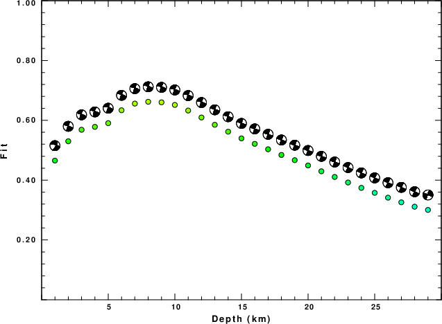
The best fit as a function of depth is given in the following figure:
|
|
Figure 2. Depth sensitivity for waveform mechanism
|
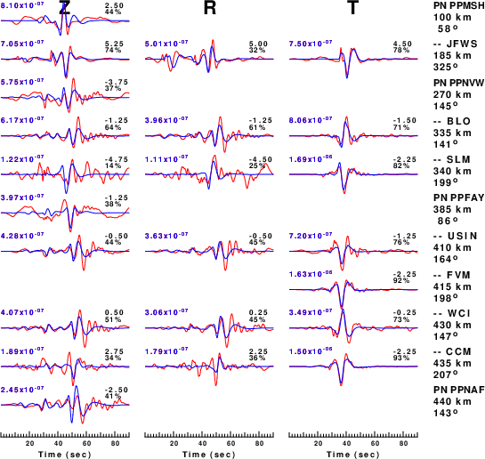
The comparison of the observed and predicted waveforms is given in the next figure. The red traces are the observed and the blue are the predicted.
Each observed-predicted component is plotted to the same scale and peak amplitudes are indicated by the numbers to the left of each trace. A pair of numbers is given in black at the right of each predicted traces. The upper number it the time shift required for maximum correlation between the observed and predicted traces. This time shift is required because the synthetics are not computed at exactly the same distance as the observed, the velocity model used in the predictions may not be perfect and the epicentral parameters may be be off.
A positive time shift indicates that the prediction is too fast and should be delayed to match the observed trace (shift to the right in this figure). A negative value indicates that the prediction is too slow. The lower number gives the percentage of variance reduction to characterize the individual goodness of fit (100% indicates a perfect fit).
The bandpass filter used in the processing and for the display was
cut o DIST/3.3 -40 o DIST/3.3 +50
rtr
taper w 0.1
hp c 0.03 n 3
lp c 0.10 n 3
|
|
Figure 3. Waveform comparison for selected depth. Red: observed; Blue - predicted. The time shift with respect to the model prediction is indicated. The percent of fit is also indicated. The time scale is relative to the first trace sample.
|
|
|
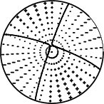
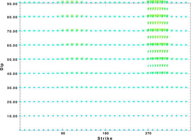
Focal mechanism sensitivity at the preferred depth. The red color indicates a very good fit to the waveforms.
Each solution is plotted as a vector at a given value of strike and dip with the angle of the vector representing the rake angle, measured, with respect to the upward vertical (N) in the figure.
|
A check on the assumed source location is possible by looking at the time shifts between the observed and predicted traces. The time shifts for waveform matching arise for several reasons:
- The origin time and epicentral distance are incorrect
- The velocity model used for the inversion is incorrect
- The velocity model used to define the P-arrival time is not the
same as the velocity model used for the waveform inversion
(assuming that the initial trace alignment is based on the
P arrival time)
Assuming only a mislocation, the time shifts are fit to a functional form:
Time_shift = A + B cos Azimuth + C Sin Azimuth
The time shifts for this inversion lead to the next figure:
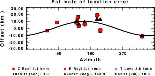
The derived shift in origin time and epicentral coordinates are given at the bottom of the figure.
Surface-Wave Focal Mechanism
The following figure shows the stations used in the grid search for the best focal mechanism to fit the surface-wave spectral amplitudes of the Love and Rayleigh waves.
|
|
Location of broadband stations used to obtain focal mechanism from surface-wave spectral amplitudes
|
The surface-wave determined focal mechanism is shown here.
  NODAL PLANES


  STK=     198.69
  DIP=      85.17
 RAKE=     164.95

             OR

  STK=     289.98
  DIP=      75.00
 RAKE=       5.00


DEPTH = 7.0 km

Mw = 4.16
Best Fit 0.7817 - P-T axis plot gives solutions with FIT greater than FIT90
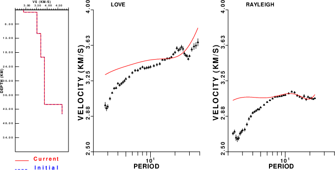
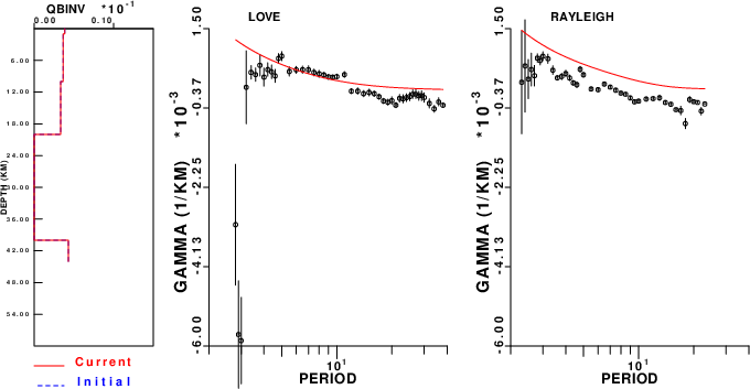
Surface-wave analysis
Surface wave analysis was performed using codes from
Computer Programs in Seismology, specifically the
multiple filter analysis program do_mft and the surface-wave
radiation pattern search program srfgrd96.
Data preparation
Digital data were collected, instrument response removed and traces converted
to Z, R an T components. Multiple filter analysis was applied to the Z and T traces to obtain the Rayleigh- and Love-wave spectral amplitudes, respectively.
These were input to the search program which examined all depths between 1 and 25 km
and all possible mechanisms.
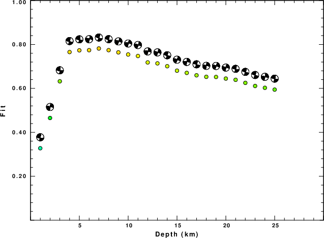
|
|
Best mechanism fit as a function of depth. The preferred depth is given above. Lower hemisphere projection
|
|
|
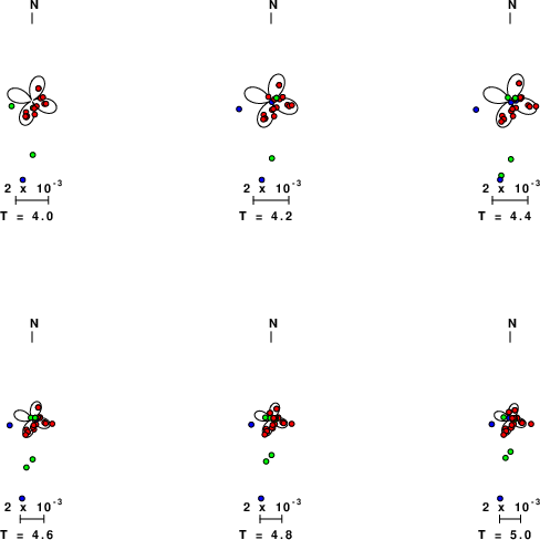
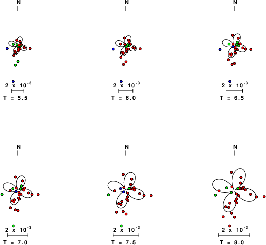
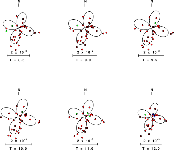
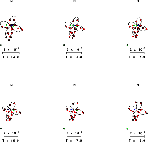
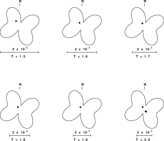
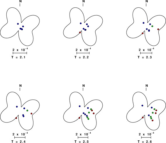
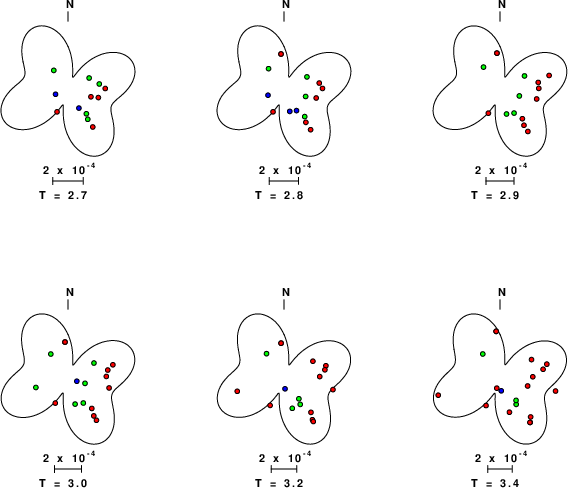
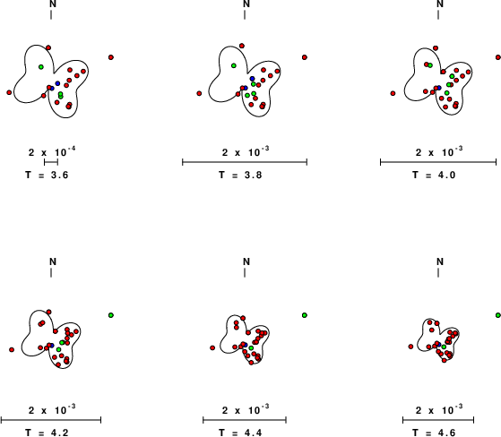
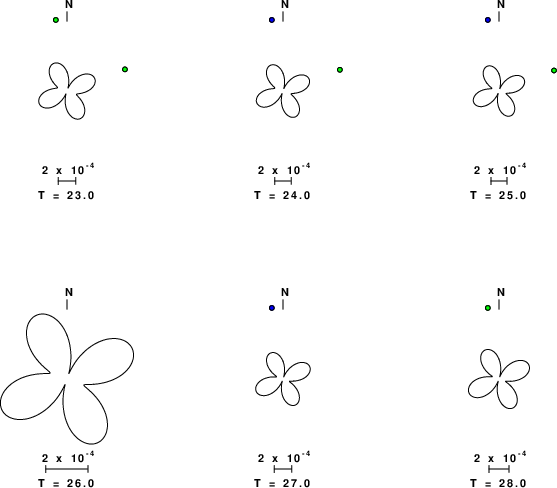
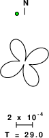
Pressure-tension axis trends. Since the surface-wave spectra search does not distinguish between P and T axes and since there is a 180 ambiguity in strike, all possible P and T axes are plotted. First motion data and waveforms will be used to select the preferred mechanism. The purpose of this plot is to provide an idea of the
possible range of solutions. The P and T-axes for all mechanisms with goodness of fit greater than 0.9 FITMAX (above) are plotted here.
|
|
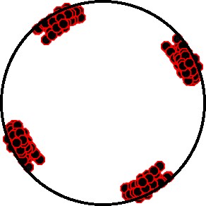
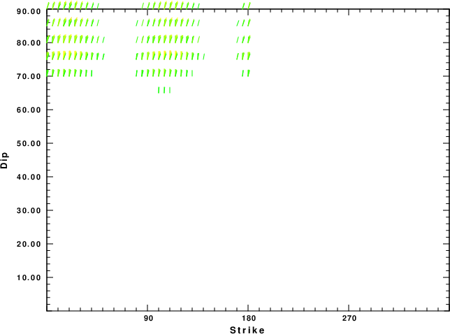
|
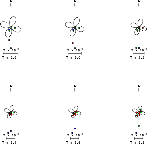
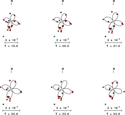
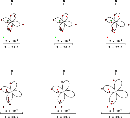
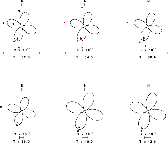
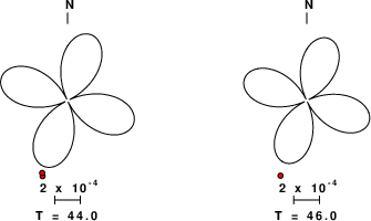
Focal mechanism sensitivity at the preferred depth. The red color indicates a very good fit to the Love and Rayleigh wave radiation patterns.
Each solution is plotted as a vector at a given value of strike and dip with the angle of the vector representing the rake angle, measured, with respect to the upward vertical (N) in the figure. Because of the symmetry of the spectral amplitude rediation patterns, only strikes from 0-180 degrees are sampled.
|
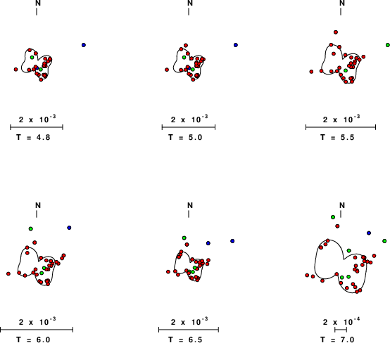
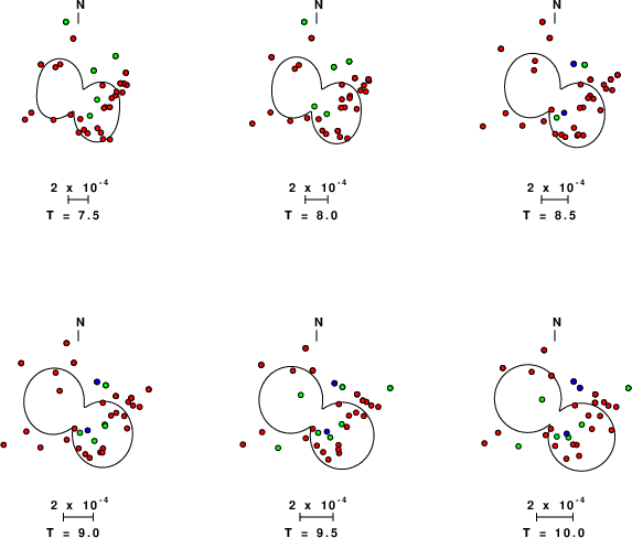
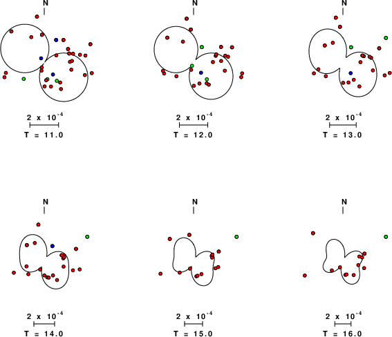
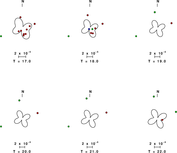
Love-wave radiation patterns
Rayleigh-wave radiation patterns