The ANSS event ID is usp000c7ec and the event page is at https://earthquake.usgs.gov/earthquakes/eventpage/usp000c7ec/executive.
2003/09/13 15:22:41 36.831 -104.907 5.0 3.8 New Mexico
 USGS/SLU Moment Tensor Solution
 ENS  2003/09/13 15:22:41:0  36.83 -104.91   5.0 3.8 New Mexico

 Stations used:
   _.ISCO IU.ANMO US.CBKS US.SDCO US.WMOK US.WUAZ UU.SRU
   XL.KNTH XL.ZIZZ

 Filtering commands used:
   cut o DIST/3.3 -40 o DIST/3.3 +50
   rtr
   taper w 0.1
   hp c 0.03 n 3
   lp c 0.10 n 3
   br c 0.12 0.25 n 4 p 2

 Best Fitting Double Couple
  Mo = 6.53e+21 dyne-cm
  Mw = 3.81
  Z  = 10 km
  Plane   Strike  Dip  Rake
   NP1      310    90    35
   NP2      220    55   180
  Principal Axes:
   Axis    Value   Plunge  Azimuth
    T   6.53e+21     24     181
    N   0.00e+00     55     310
    P  -6.53e+21     24      79

 Moment Tensor: (dyne-cm)
    Component   Value
       Mxx     5.27e+21
       Mxy    -9.29e+20
       Mxz    -2.87e+21
       Myy    -5.27e+21
       Myz    -2.41e+21
       Mzz    -3.28e+14


                     ##############
                 ######################
              #######################-----
             ###################-----------
           ---##############-----------------
          ------##########--------------------
         ---------######-----------------------
        ------------##--------------------------
        ------------##--------------------   ---
       ------------######----------------- P ----
       -----------#########---------------   ----
       ----------############--------------------
       ---------###############------------------
        -------###################--------------
        -------#####################------------
         -----########################---------
          ----##########################------
           ---############################---
             -############   ##############
              -########### T #############
                 #########   ##########
                     ##############


 Global CMT Convention Moment Tensor:
      R          T          P
 -3.28e+14  -2.87e+21   2.41e+21
 -2.87e+21   5.27e+21   9.29e+20
  2.41e+21   9.29e+20  -5.27e+21


Details of the solution is found at

http://www.eas.slu.edu/eqc/eqc_mt/MECH.NA/20030913152241/index.html
|
      STK = 310
      DIP = 90
     RAKE = 35
       MW = 3.81
       HS = 10.0
The NDK file is 20030913152241.ndk The waveform inversion is preferred.
|
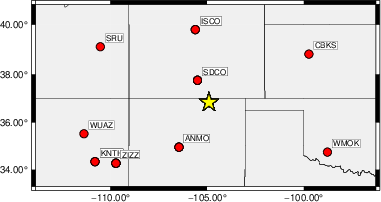
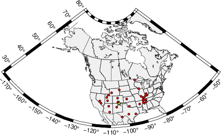
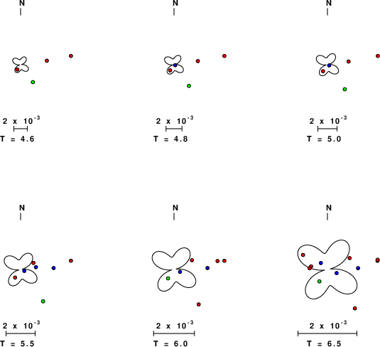
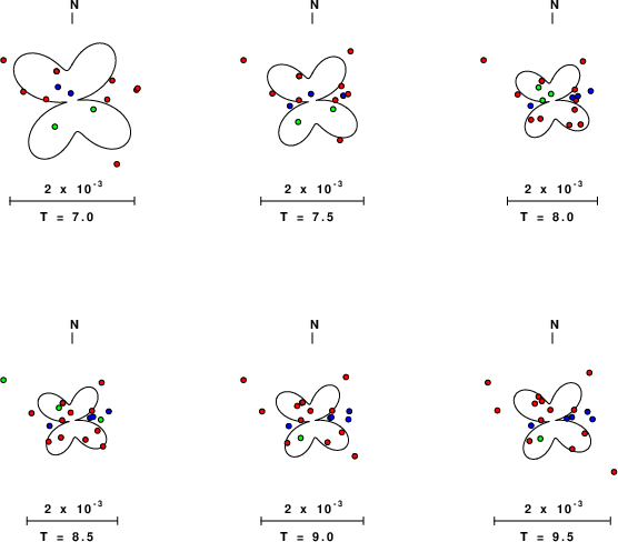
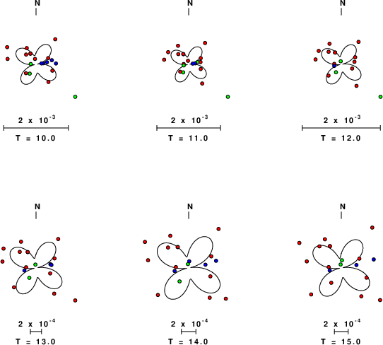
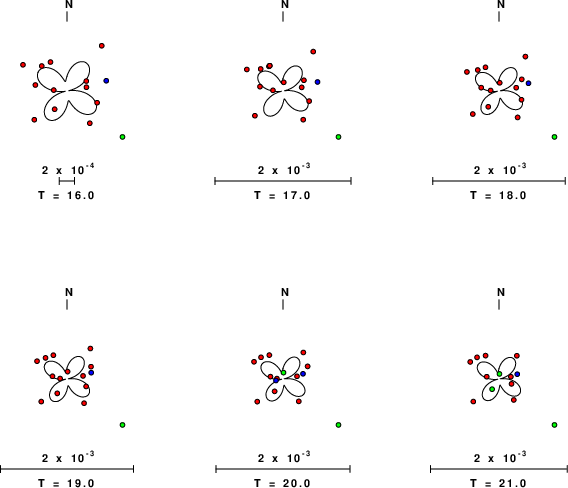
The focal mechanism was determined using broadband seismic waveforms. The location of the event (star) and the stations used for (red) the waveform inversion are shown in the next figure.
|
|
|
The program wvfgrd96 was used with good traces observed at short distance to determine the focal mechanism, depth and seismic moment. This technique requires a high quality signal and well determined velocity model for the Green's functions. To the extent that these are the quality data, this type of mechanism should be preferred over the radiation pattern technique which requires the separate step of defining the pressure and tension quadrants and the correct strike.
The observed and predicted traces are filtered using the following gsac commands:
cut o DIST/3.3 -40 o DIST/3.3 +50
rtr
taper w 0.1
hp c 0.03 n 3
lp c 0.10 n 3
br c 0.12 0.25 n 4 p 2
The results of this grid search are as follow:
           DEPTH  STK   DIP  RAKE   MW    FIT
WVFGRD96    1.0   305    70    20   3.47 0.3347
WVFGRD96    2.0   315    60    30   3.64 0.5191
WVFGRD96    3.0   310    70    20   3.65 0.5772
WVFGRD96    4.0   310    85    25   3.67 0.6238
WVFGRD96    5.0   125    85   -30   3.72 0.6574
WVFGRD96    6.0   120    60   -40   3.75 0.6735
WVFGRD96    7.0   120    65   -35   3.77 0.6922
WVFGRD96    8.0   130    90   -40   3.79 0.6915
WVFGRD96    9.0   130    90   -40   3.81 0.6995
WVFGRD96   10.0   310    90    35   3.81 0.7036
WVFGRD96   11.0   310    90    35   3.82 0.7028
WVFGRD96   12.0   130    90   -25   3.82 0.7018
WVFGRD96   13.0   310    90    25   3.83 0.7016
WVFGRD96   14.0   130    85   -25   3.84 0.7002
WVFGRD96   15.0   315    85    25   3.84 0.6972
WVFGRD96   16.0   130    85   -25   3.86 0.6974
WVFGRD96   17.0   135    90   -25   3.86 0.6984
WVFGRD96   18.0   315    90    25   3.87 0.6981
WVFGRD96   19.0   135    90   -25   3.88 0.6981
WVFGRD96   20.0   135    85   -25   3.89 0.6985
WVFGRD96   21.0   135    85   -25   3.90 0.6989
WVFGRD96   22.0   135    85   -25   3.91 0.6988
WVFGRD96   23.0   135    85   -20   3.91 0.7006
WVFGRD96   24.0   135    80   -25   3.93 0.7015
WVFGRD96   25.0   135    80   -25   3.94 0.7009
WVFGRD96   26.0   135    80   -25   3.94 0.6980
WVFGRD96   27.0   135    80   -25   3.95 0.6927
WVFGRD96   28.0   135    80   -25   3.96 0.6874
WVFGRD96   29.0   135    80   -25   3.97 0.6800
The best solution is
WVFGRD96 10.0 310 90 35 3.81 0.7036
The mechanism corresponding to the best fit is
|
|
|
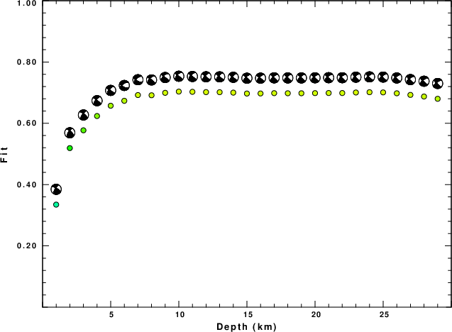
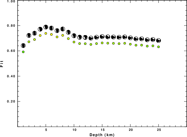
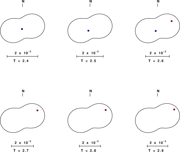
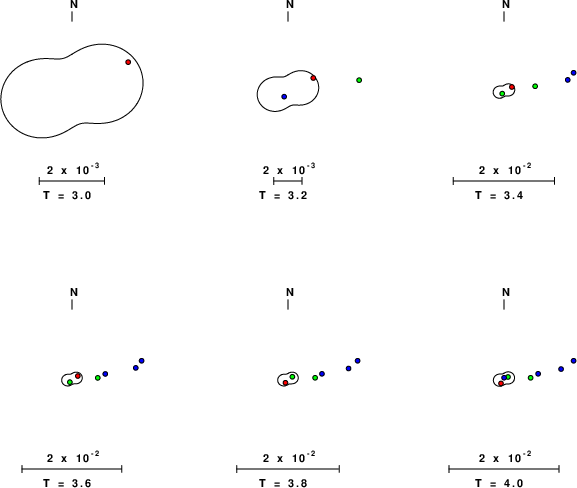
The best fit as a function of depth is given in the following figure:
|
|
|
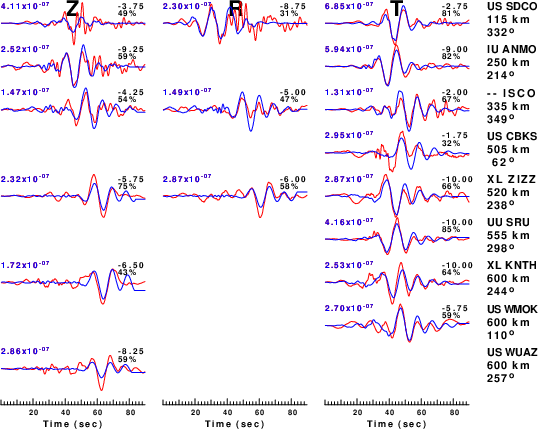
The comparison of the observed and predicted waveforms is given in the next figure. The red traces are the observed and the blue are the predicted. Each observed-predicted component is plotted to the same scale and peak amplitudes are indicated by the numbers to the left of each trace. A pair of numbers is given in black at the right of each predicted traces. The upper number it the time shift required for maximum correlation between the observed and predicted traces. This time shift is required because the synthetics are not computed at exactly the same distance as the observed, the velocity model used in the predictions may not be perfect and the epicentral parameters may be be off. A positive time shift indicates that the prediction is too fast and should be delayed to match the observed trace (shift to the right in this figure). A negative value indicates that the prediction is too slow. The lower number gives the percentage of variance reduction to characterize the individual goodness of fit (100% indicates a perfect fit).
The bandpass filter used in the processing and for the display was
cut o DIST/3.3 -40 o DIST/3.3 +50
rtr
taper w 0.1
hp c 0.03 n 3
lp c 0.10 n 3
br c 0.12 0.25 n 4 p 2
|
| Figure 3. Waveform comparison for selected depth. Red: observed; Blue - predicted. The time shift with respect to the model prediction is indicated. The percent of fit is also indicated. The time scale is relative to the first trace sample. |
|
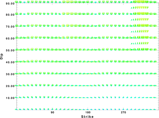
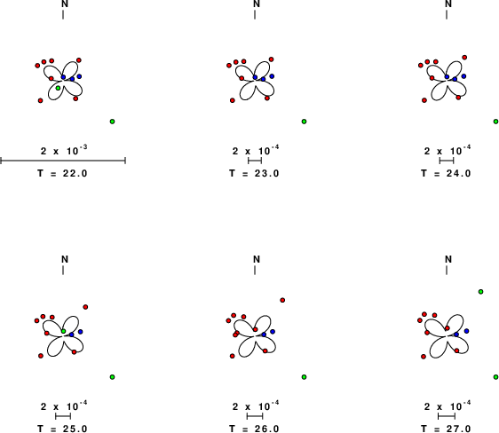
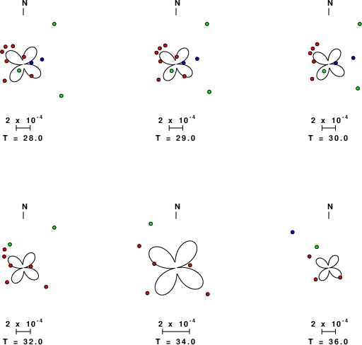
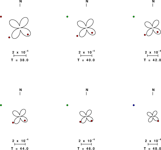
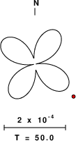
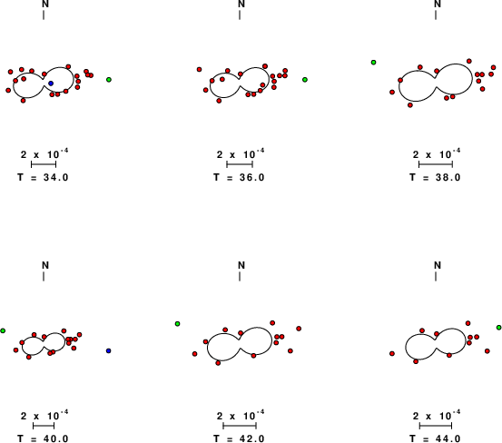
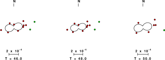
| Focal mechanism sensitivity at the preferred depth. The red color indicates a very good fit to the waveforms. Each solution is plotted as a vector at a given value of strike and dip with the angle of the vector representing the rake angle, measured, with respect to the upward vertical (N) in the figure. |
A check on the assumed source location is possible by looking at the time shifts between the observed and predicted traces. The time shifts for waveform matching arise for several reasons:
Time_shift = A + B cos Azimuth + C Sin Azimuth
The time shifts for this inversion lead to the next figure:
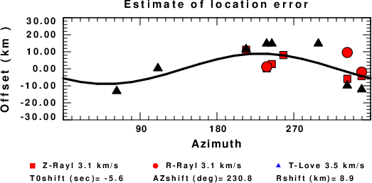
The derived shift in origin time and epicentral coordinates are given at the bottom of the figure.
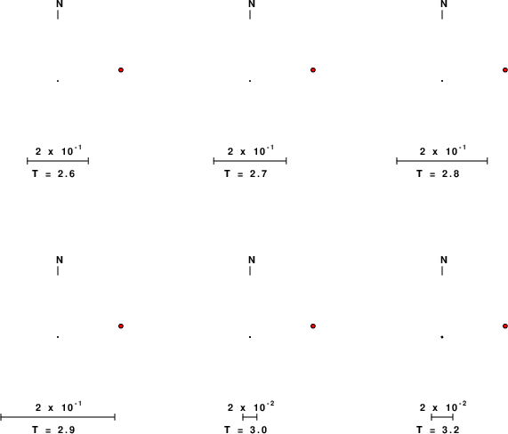
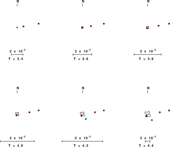
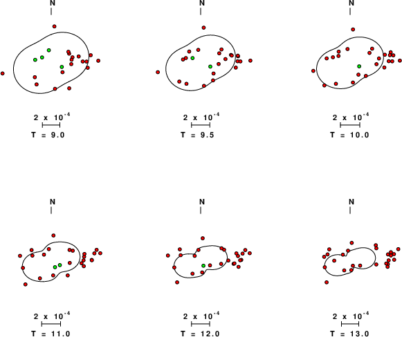
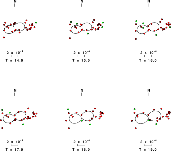
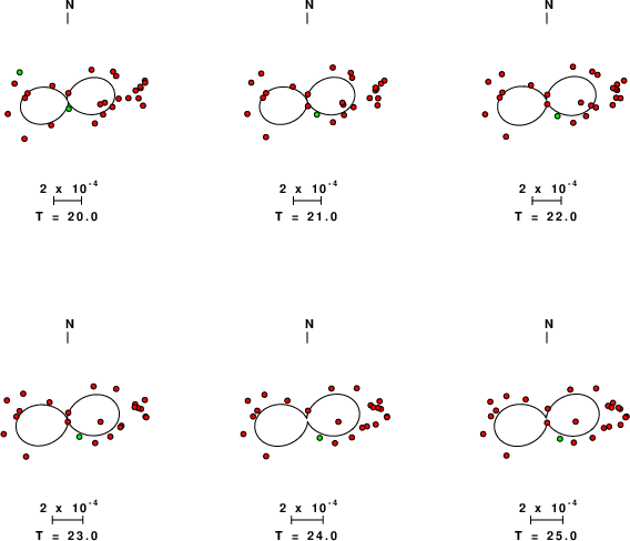
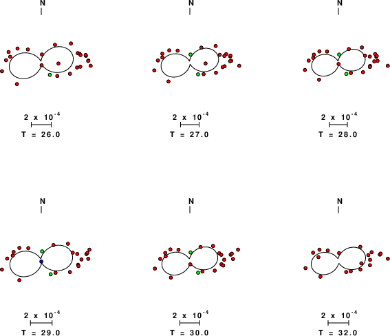
The following figure shows the stations used in the grid search for the best focal mechanism to fit the surface-wave spectral amplitudes of the Love and Rayleigh waves.
|
|
|
The surface-wave determined focal mechanism is shown here.
  NODAL PLANES


  STK=     164.99
  DIP=      60.00
 RAKE=     -94.99

             OR

  STK=     354.90
  DIP=      30.38
 RAKE=     -81.43


DEPTH = 05.0 km

Mw = 3.98
Best Fit 0.7383 - P-T axis plot gives solutions with FIT greater than FIT90
 |
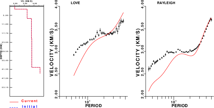
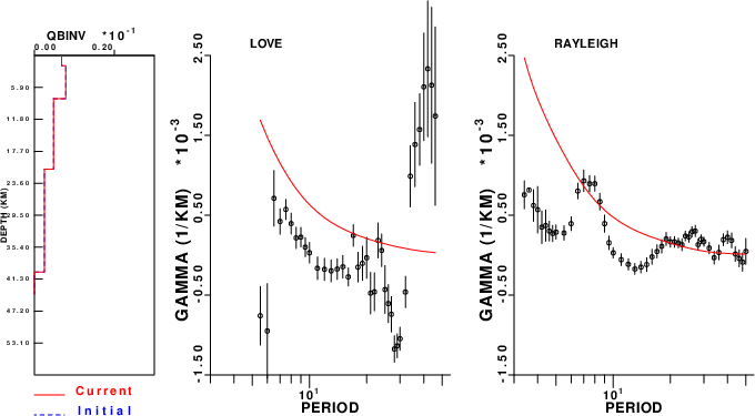
Surface wave analysis was performed using codes from Computer Programs in Seismology, specifically the multiple filter analysis program do_mft and the surface-wave radiation pattern search program srfgrd96.
Digital data were collected, instrument response removed and traces converted
to Z, R an T components. Multiple filter analysis was applied to the Z and T traces to obtain the Rayleigh- and Love-wave spectral amplitudes, respectively.
These were input to the search program which examined all depths between 1 and 25 km
and all possible mechanisms.
|
|
|
|
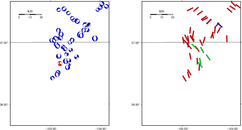
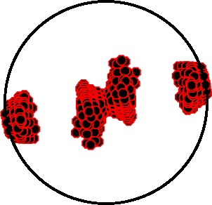
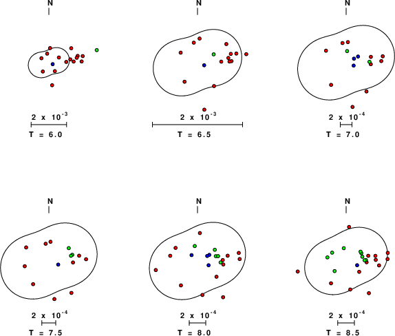
| Pressure-tension axis trends. Since the surface-wave spectra search does not distinguish between P and T axes and since there is a 180 ambiguity in strike, all possible P and T axes are plotted. First motion data and waveforms will be used to select the preferred mechanism. The purpose of this plot is to provide an idea of the possible range of solutions. The P and T-axes for all mechanisms with goodness of fit greater than 0.9 FITMAX (above) are plotted here. |
|
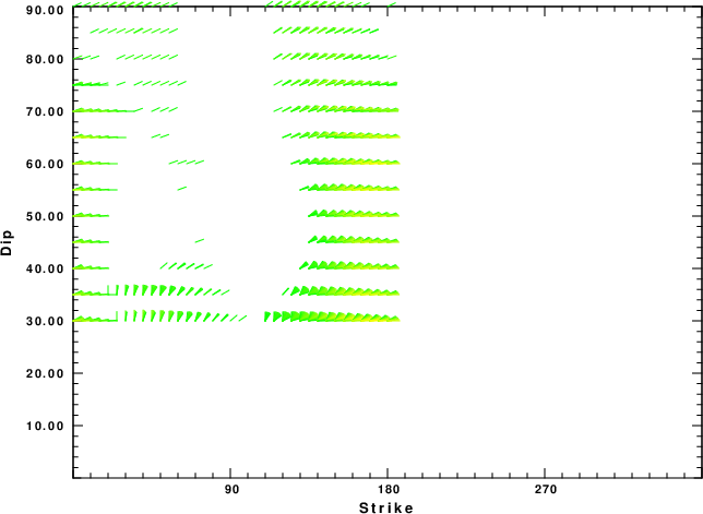
| Focal mechanism sensitivity at the preferred depth. The red color indicates a very good fit to the Love and Rayleigh wave radiation patterns. Each solution is plotted as a vector at a given value of strike and dip with the angle of the vector representing the rake angle, measured, with respect to the upward vertical (N) in the figure. Because of the symmetry of the spectral amplitude rediation patterns, only strikes from 0-180 degrees are sampled. |
|
|
The WUS.model used for the waveform synthetic seismograms and for the surface wave eigenfunctions and dispersion is as follows (The format is in the model96 format of Computer Programs in Seismology).
MODEL.01
Model after     8 iterations
ISOTROPIC
KGS
FLAT EARTH
1-D
CONSTANT VELOCITY
LINE08
LINE09
LINE10
LINE11
      H(KM)   VP(KM/S)   VS(KM/S) RHO(GM/CC)         QP         QS       ETAP       ETAS      FREFP      FREFS
     1.9000     3.4065     2.0089     2.2150  0.302E-02  0.679E-02   0.00       0.00       1.00       1.00
     6.1000     5.5445     3.2953     2.6089  0.349E-02  0.784E-02   0.00       0.00       1.00       1.00
    13.0000     6.2708     3.7396     2.7812  0.212E-02  0.476E-02   0.00       0.00       1.00       1.00
    19.0000     6.4075     3.7680     2.8223  0.111E-02  0.249E-02   0.00       0.00       1.00       1.00
     0.0000     7.9000     4.6200     3.2760  0.164E-10  0.370E-10   0.00       0.00       1.00       1.00