Location

Location ANSS

The ANSS event ID is uw10555268 and the event page is at https://earthquake.usgs.gov/earthquakes/eventpage/uw10555268/executive.

2002/05/15 17:54:48 42.231 -121.901 6.3 4.3 Oregon

Focal Mechanism

USGS/SLU Moment Tensor Solution ENS 2002/05/15 17:54:48:0 42.23 -121.90 6.3 4.3 Oregon Stations used: BK.CMB CI.MLAC LB.BMN LB.TPH US.ELK US.HLID US.MNV US.WVOR UW.TAKO YS.GPSS1 Filtering commands used: hp c 0.02 n 3 lp c 0.06 n 3 Best Fitting Double Couple Mo = 2.19e+22 dyne-cm Mw = 4.16 Z = 12 km Plane Strike Dip Rake NP1 144 73 115 NP2 265 30 35 Principal Axes: Axis Value Plunge Azimuth T 2.19e+22 55 85 N 0.00e+00 24 316 P -2.19e+22 24 214 Moment Tensor: (dyne-cm) Component Value Mxx -1.23e+22 Mxy -7.88e+21 Mxz 7.60e+21 Myy 1.47e+21 Myz 1.49e+22 Mzz 1.09e+22 -------------- ---------------------- ##-------------------------- ###-------############-------- ######-######################----- #####--#########################---- ####-----##########################--- ###--------###########################-- ##----------###########################- ##------------############## ##########- #--------------############# T ########### #---------------############ ########### ------------------######################## ------------------###################### --------------------#################### --------------------################## ---------------------############### ------ -------------############ ---- P ---------------######## --- ------------------#### ---------------------- -------------- Global CMT Convention Moment Tensor: R T P 1.09e+22 7.60e+21 -1.49e+22 7.60e+21 -1.23e+22 7.88e+21 -1.49e+22 7.88e+21 1.47e+21 Details of the solution is found at http://www.eas.slu.edu/eqc/eqc_mt/MECH.NA/20020515175448/index.html

Preferred Solution

      STK = 265
      DIP = 30
     RAKE = 35
       MW = 4.16
       HS = 12.0

The NDK file is 20020515175448.ndk The waveform inversion is preferred.

Context

Waveform Inversion using wvfgrd96

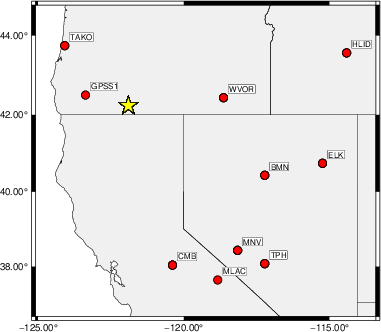
The focal mechanism was determined using broadband seismic waveforms. The location of the event (star) and the stations used for (red) the waveform inversion are shown in the next figure.

Location of broadband stations used for waveform inversion

The program wvfgrd96 was used with good traces observed at short distance to determine the focal mechanism, depth and seismic moment. This technique requires a high quality signal and well determined velocity model for the Green's functions. To the extent that these are the quality data, this type of mechanism should be preferred over the radiation pattern technique which requires the separate step of defining the pressure and tension quadrants and the correct strike.

The observed and predicted traces are filtered using the following gsac commands:

hp c 0.02 n 3
lp c 0.06 n 3

           DEPTH  STK   DIP  RAKE   MW    FIT
WVFGRD96    0.5   330    40  -100   3.88 0.4638
WVFGRD96    1.0   210    60   -60   3.86 0.4643
WVFGRD96    2.0   210    60   -60   3.94 0.4973
WVFGRD96    3.0   215    65   -60   4.00 0.4634
WVFGRD96    4.0    10    80   -65   4.06 0.4300
WVFGRD96    5.0   245    20     0   4.08 0.4840
WVFGRD96    6.0   250    25     5   4.07 0.5237
WVFGRD96    7.0   250    25     5   4.07 0.5497
WVFGRD96    8.0   240    20   -10   4.13 0.5641
WVFGRD96    9.0   250    25     5   4.13 0.5769
WVFGRD96   10.0   255    25    15   4.13 0.5829
WVFGRD96   11.0   260    30    30   4.15 0.5854
WVFGRD96   12.0   265    30    35   4.16 0.5868
WVFGRD96   13.0   265    30    35   4.16 0.5856
WVFGRD96   14.0   265    30    35   4.16 0.5815
WVFGRD96   15.0   270    30    40   4.16 0.5766
WVFGRD96   16.0   270    30    40   4.17 0.5701
WVFGRD96   17.0   270    30    40   4.17 0.5627
WVFGRD96   18.0   270    30    40   4.17 0.5543
WVFGRD96   19.0   270    30    40   4.18 0.5456
WVFGRD96   20.0   270    30    40   4.18 0.5366
WVFGRD96   21.0   275    30    45   4.20 0.5277
WVFGRD96   22.0   275    30    45   4.20 0.5179
WVFGRD96   23.0   275    30    45   4.20 0.5078
WVFGRD96   24.0   275    30    45   4.21 0.4975
WVFGRD96   25.0   275    30    45   4.21 0.4868
WVFGRD96   26.0   285    25    55   4.22 0.4758
WVFGRD96   27.0   285    25    55   4.23 0.4647
WVFGRD96   28.0   285    25    55   4.23 0.4533
WVFGRD96   29.0   285    25    55   4.23 0.4414

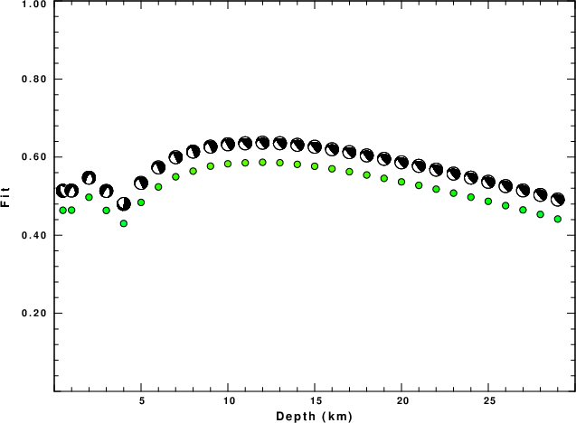
The best solution is

WVFGRD96   12.0   265    30    35   4.16 0.5868

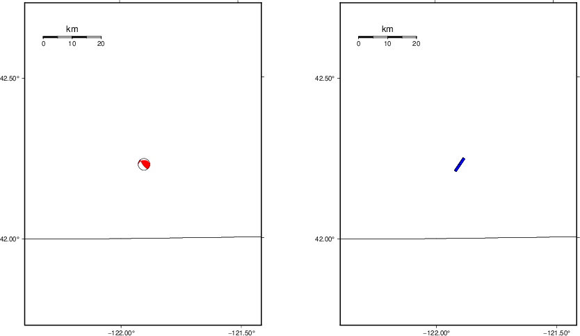
The mechanism corresponding to the best fit is

Figure 1. Waveform inversion focal mechanism

The best fit as a function of depth is given in the following figure:

Figure 2. Depth sensitivity for waveform mechanism

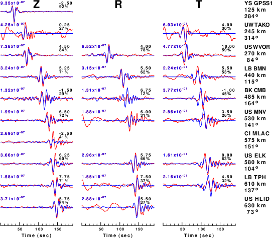
The comparison of the observed and predicted waveforms is given in the next figure. The red traces are the observed and the blue are the predicted. Each observed-predicted component is plotted to the same scale and peak amplitudes are indicated by the numbers to the left of each trace. A pair of numbers is given in black at the right of each predicted traces. The upper number it the time shift required for maximum correlation between the observed and predicted traces. This time shift is required because the synthetics are not computed at exactly the same distance as the observed, the velocity model used in the predictions may not be perfect and the epicentral parameters may be be off. A positive time shift indicates that the prediction is too fast and should be delayed to match the observed trace (shift to the right in this figure). A negative value indicates that the prediction is too slow. The lower number gives the percentage of variance reduction to characterize the individual goodness of fit (100% indicates a perfect fit).

The bandpass filter used in the processing and for the display was

hp c 0.02 n 3
lp c 0.06 n 3

Figure 3. Waveform comparison for selected depth. Red: observed; Blue - predicted. The time shift with respect to the model prediction is indicated. The percent of fit is also indicated. The time scale is relative to the first trace sample.

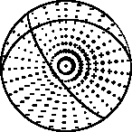
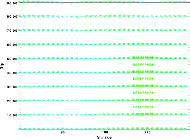
Focal mechanism sensitivity at the preferred depth. The red color indicates a very good fit to the waveforms. Each solution is plotted as a vector at a given value of strike and dip with the angle of the vector representing the rake angle, measured, with respect to the upward vertical (N) in the figure.

A check on the assumed source location is possible by looking at the time shifts between the observed and predicted traces. The time shifts for waveform matching arise for several reasons:

• The origin time and epicentral distance are incorrect
• The velocity model used for the inversion is incorrect
• The velocity model used to define the P-arrival time is not the same as the velocity model used for the waveform inversion (assuming that the initial trace alignment is based on the P arrival time)

 Time_shift = A + B cos Azimuth + C Sin Azimuth

The time shifts for this inversion lead to the next figure:

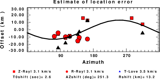
The derived shift in origin time and epicentral coordinates are given at the bottom of the figure.

Velocity Model

The WUS.model used for the waveform synthetic seismograms and for the surface wave eigenfunctions and dispersion is as follows (The format is in the model96 format of Computer Programs in Seismology).

MODEL.01
Model after     8 iterations
ISOTROPIC
KGS
FLAT EARTH
1-D
CONSTANT VELOCITY
LINE08
LINE09
LINE10
LINE11
      H(KM)   VP(KM/S)   VS(KM/S) RHO(GM/CC)         QP         QS       ETAP       ETAS      FREFP      FREFS
     1.9000     3.4065     2.0089     2.2150  0.302E-02  0.679E-02   0.00       0.00       1.00       1.00    
     6.1000     5.5445     3.2953     2.6089  0.349E-02  0.784E-02   0.00       0.00       1.00       1.00    
    13.0000     6.2708     3.7396     2.7812  0.212E-02  0.476E-02   0.00       0.00       1.00       1.00    
    19.0000     6.4075     3.7680     2.8223  0.111E-02  0.249E-02   0.00       0.00       1.00       1.00    
     0.0000     7.9000     4.6200     3.2760  0.164E-10  0.370E-10   0.00       0.00       1.00       1.00