The ANSS event ID is ld2002042000 and the event page is at https://earthquake.usgs.gov/earthquakes/eventpage/ld2002042000/executive.
2002/04/20 10:50:44 44.512 -73.697 4.8 5.3 New York
 USGS/SLU Moment Tensor Solution
 ENS  2002/04/20 10:50:44:0  44.51  -73.70   4.8 5.3 New York

 Stations used:
   CN.A54 CN.A61 CN.A64 CN.GAC CN.KGNO CN.LMQ CN.MNT CN.SADO
   CN.VLDQ IU.HRV IU.SSPA LD.ACCN LD.BRNJ LD.CONY LD.CPNY
   LD.MVL LD.PAL LD.SDMD PO.ELGO US.BINY US.LBNH US.NCB

 Filtering commands used:
   cut o DIST/3.3 -40 o DIST/3.3 +50
   rtr
   taper w 0.1
   hp c 0.03 n 3
   lp c 0.10 n 3

 Best Fitting Double Couple
  Mo = 2.37e+23 dyne-cm
  Mw = 4.85
  Z  = 11 km
  Plane   Strike  Dip  Rake
   NP1      187    56    97
   NP2      355    35    80
  Principal Axes:
   Axis    Value   Plunge  Azimuth
    T   2.37e+23     78     122
    N   0.00e+00      6       3
    P  -2.37e+23     10     272

 Moment Tensor: (dyne-cm)
    Component   Value
       Mxx     2.43e+21
       Mxy     4.21e+21
       Mxz    -2.66e+22
       Myy    -2.22e+23
       Myz     8.25e+22
       Mzz     2.19e+23


                     --------#-----
                 ----------######------
              -----------##########-------
             -----------#############------
           ------------###############-------
          ------------#################-------
         ------------###################-------
        -------------###################--------
        ------------#####################-------
       -   ---------#####################--------
       - P --------#########   ###########-------
       -   --------######### T ###########-------
       ------------#########   ###########-------
        -----------######################-------
        -----------######################-------
         -----------####################-------
          ----------####################------
           ---------###################------
             --------#################-----
              --------##############------
                 ------############----
                     ---########---


 Global CMT Convention Moment Tensor:
      R          T          P
  2.19e+23  -2.66e+22  -8.25e+22
 -2.66e+22   2.43e+21  -4.21e+21
 -8.25e+22  -4.21e+21  -2.22e+23


Details of the solution is found at

http://www.eas.slu.edu/eqc/eqc_mt/MECH.NA/20020420105044/index.html
|
      STK = -5
      DIP = 35
     RAKE = 80
       MW = 4.85
       HS = 11.0
The NDK file is 20020420105044.ndk The waveform inversion is preferred.
The following compares this source inversion to those provided by others. The purpose is to look for major differences and also to note slight differences that might be inherent to the processing procedure. For completeness the USGS/SLU solution is repeated from above.
 USGS/SLU Moment Tensor Solution
 ENS  2002/04/20 10:50:44:0  44.51  -73.70   4.8 5.3 New York

 Stations used:
   CN.A54 CN.A61 CN.A64 CN.GAC CN.KGNO CN.LMQ CN.MNT CN.SADO
   CN.VLDQ IU.HRV IU.SSPA LD.ACCN LD.BRNJ LD.CONY LD.CPNY
   LD.MVL LD.PAL LD.SDMD PO.ELGO US.BINY US.LBNH US.NCB

 Filtering commands used:
   cut o DIST/3.3 -40 o DIST/3.3 +50
   rtr
   taper w 0.1
   hp c 0.03 n 3
   lp c 0.10 n 3

 Best Fitting Double Couple
  Mo = 2.37e+23 dyne-cm
  Mw = 4.85
  Z  = 11 km
  Plane   Strike  Dip  Rake
   NP1      187    56    97
   NP2      355    35    80
  Principal Axes:
   Axis    Value   Plunge  Azimuth
    T   2.37e+23     78     122
    N   0.00e+00      6       3
    P  -2.37e+23     10     272

 Moment Tensor: (dyne-cm)
    Component   Value
       Mxx     2.43e+21
       Mxy     4.21e+21
       Mxz    -2.66e+22
       Myy    -2.22e+23
       Myz     8.25e+22
       Mzz     2.19e+23


                     --------#-----
                 ----------######------
              -----------##########-------
             -----------#############------
           ------------###############-------
          ------------#################-------
         ------------###################-------
        -------------###################--------
        ------------#####################-------
       -   ---------#####################--------
       - P --------#########   ###########-------
       -   --------######### T ###########-------
       ------------#########   ###########-------
        -----------######################-------
        -----------######################-------
         -----------####################-------
          ----------####################------
           ---------###################------
             --------#################-----
              --------##############------
                 ------############----
                     ---########---


 Global CMT Convention Moment Tensor:
      R          T          P
  2.19e+23  -2.66e+22  -8.25e+22
 -2.66e+22   2.43e+21  -4.21e+21
 -8.25e+22  -4.21e+21  -2.22e+23


Details of the solution is found at

http://www.eas.slu.edu/eqc/eqc_mt/MECH.NA/20020420105044/index.html
|
REVISED Quick CMT:

04/20/2002, 10:50:44, NEW YORK, Mw=5.0

The following is a REVISED solution for the April 20, 2002,
event in New York. This CMT solution was determined by
analysis of long-period body waves (45-150 s) and
intermediate-period surface waves (40-100 s or 50-200 s).
A preliminary very-broad-band analysis of teleseismic
P waveforms gives a depth for this event of 10.4 km.

Here is the solution for the recent event.

April 20, 2002, NEW YORK, Mw=5.0

Meredith Nettles
Mike Antolik

CENTROID, MOMENT TENSOR SOLUTION
HARVARD EVENT-FILE NAME S042002A
DATA USED: GSN
L.P. BODY WAVES: 23S, 38C, T= 45
SURFACE WAVES:   27S, 58C, T= 40
CENTROID LOCATION:
ORIGIN TIME       10:50:48.2 0.2
LAT 44.69N 0.01;LON  73.80W 0.02
DEP   8.9 0.8;HALF-DURATION  1.4
MOMENT TENSOR; SCALE 10**23 D-CM
  MRR= 3.19 0.17; MTT= 0.10 0.08
  MFF=-3.29 0.10; MRT=-1.45 0.25
  MRF=-0.46 0.18; MTF=-0.13 0.04
 PRINCIPAL AXES:
 1.(T) VAL=  3.78;PLG=68;AZM=172
 2.(N)      -0.44;    21;      6
 3.(P)      -3.34;     5;    274
BEST DOUBLE COUPLE:M0=3.6*10**23
 NP1:STRIKE=343;DIP=44;SLIP=  59
 NP2:       203;    53;      116

            --#########
        ----------##-------
      -----------###---------
    -----------#######---------
   -----------##########--------
  -----------############--------
  ----------##############-------
   --------###############--------
 P -------#################-------
   ------##################-------
 --------########   #######-------
  -------######## T #######------
  -------########   #######------
   ------##################-----
    -----#################-----
      ----###############----
        --##############---
            ###########
|
|
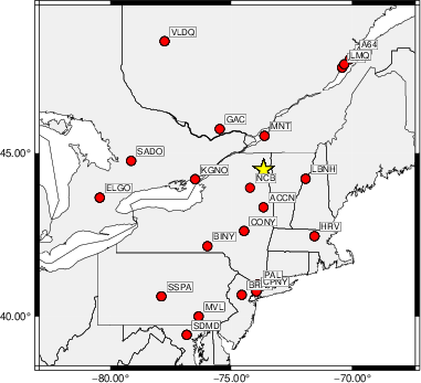
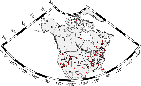
The focal mechanism was determined using broadband seismic waveforms. The location of the event (star) and the stations used for (red) the waveform inversion are shown in the next figure.
|
|
|
The program wvfgrd96 was used with good traces observed at short distance to determine the focal mechanism, depth and seismic moment. This technique requires a high quality signal and well determined velocity model for the Green's functions. To the extent that these are the quality data, this type of mechanism should be preferred over the radiation pattern technique which requires the separate step of defining the pressure and tension quadrants and the correct strike.
The observed and predicted traces are filtered using the following gsac commands:
cut o DIST/3.3 -40 o DIST/3.3 +50
rtr
taper w 0.1
hp c 0.03 n 3
lp c 0.10 n 3
The results of this grid search are as follow:
           DEPTH  STK   DIP  RAKE   MW    FIT
WVFGRD96    1.0     0    55   -90   4.72 0.5592
WVFGRD96    2.0    25    20   -50   4.81 0.5016
WVFGRD96    3.0    20    20   -55   4.76 0.5069
WVFGRD96    4.0   325    35    15   4.72 0.5232
WVFGRD96    5.0   345    30    60   4.78 0.5797
WVFGRD96    6.0   355    30    75   4.80 0.6449
WVFGRD96    7.0   355    35    75   4.81 0.7011
WVFGRD96    8.0   355    35    75   4.81 0.7397
WVFGRD96    9.0   355    35    80   4.82 0.7634
WVFGRD96   10.0   355    35    80   4.85 0.7743
WVFGRD96   11.0    -5    35    80   4.85 0.7802
WVFGRD96   12.0   355    35    80   4.85 0.7773
WVFGRD96   13.0   355    35    80   4.85 0.7671
WVFGRD96   14.0   350    35    75   4.85 0.7520
WVFGRD96   15.0   350    35    70   4.85 0.7335
WVFGRD96   16.0   350    35    70   4.86 0.7124
WVFGRD96   17.0   350    35    70   4.86 0.6887
WVFGRD96   18.0   355    45    80   4.86 0.6633
WVFGRD96   19.0    -5    45    80   4.87 0.6397
WVFGRD96   20.0     0    50    85   4.90 0.6186
WVFGRD96   21.0     0    50    85   4.90 0.5978
WVFGRD96   22.0   185    40    95   4.91 0.5770
WVFGRD96   23.0   185    35    95   4.91 0.5544
WVFGRD96   24.0     0    55    90   4.91 0.5316
WVFGRD96   25.0     0    55    90   4.92 0.5086
WVFGRD96   26.0     0    55    90   4.92 0.4841
WVFGRD96   27.0   185    35    95   4.93 0.4590
WVFGRD96   28.0   185    30    95   4.93 0.4336
WVFGRD96   29.0     0    60    90   4.93 0.4083
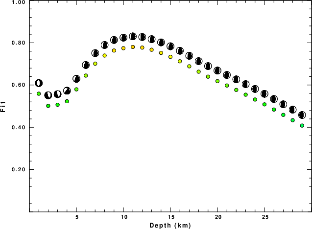
The best solution is
WVFGRD96 11.0 -5 35 80 4.85 0.7802
The mechanism corresponding to the best fit is
|
|
|
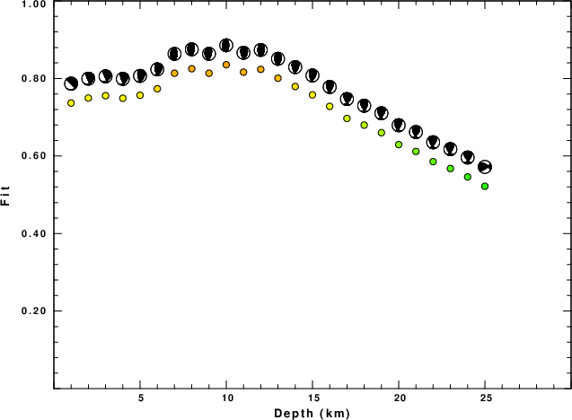
The best fit as a function of depth is given in the following figure:
|
|
|
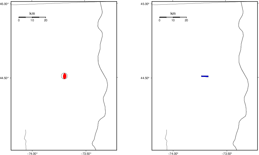
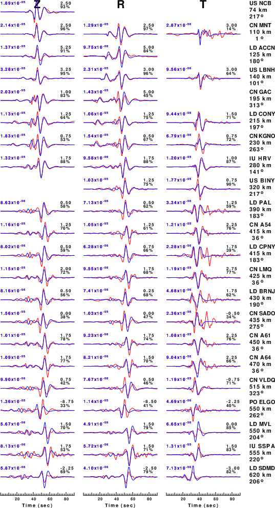
The comparison of the observed and predicted waveforms is given in the next figure. The red traces are the observed and the blue are the predicted. Each observed-predicted component is plotted to the same scale and peak amplitudes are indicated by the numbers to the left of each trace. A pair of numbers is given in black at the right of each predicted traces. The upper number it the time shift required for maximum correlation between the observed and predicted traces. This time shift is required because the synthetics are not computed at exactly the same distance as the observed, the velocity model used in the predictions may not be perfect and the epicentral parameters may be be off. A positive time shift indicates that the prediction is too fast and should be delayed to match the observed trace (shift to the right in this figure). A negative value indicates that the prediction is too slow. The lower number gives the percentage of variance reduction to characterize the individual goodness of fit (100% indicates a perfect fit).
The bandpass filter used in the processing and for the display was
cut o DIST/3.3 -40 o DIST/3.3 +50
rtr
taper w 0.1
hp c 0.03 n 3
lp c 0.10 n 3
|
| Figure 3. Waveform comparison for selected depth. Red: observed; Blue - predicted. The time shift with respect to the model prediction is indicated. The percent of fit is also indicated. The time scale is relative to the first trace sample. |
|
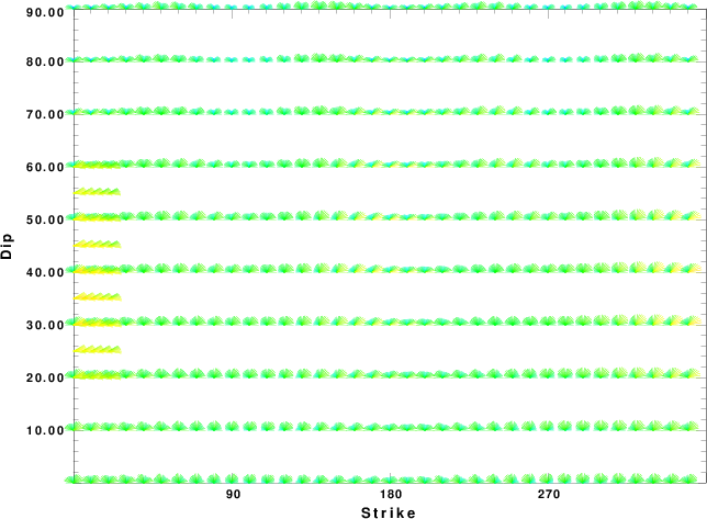
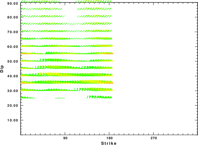
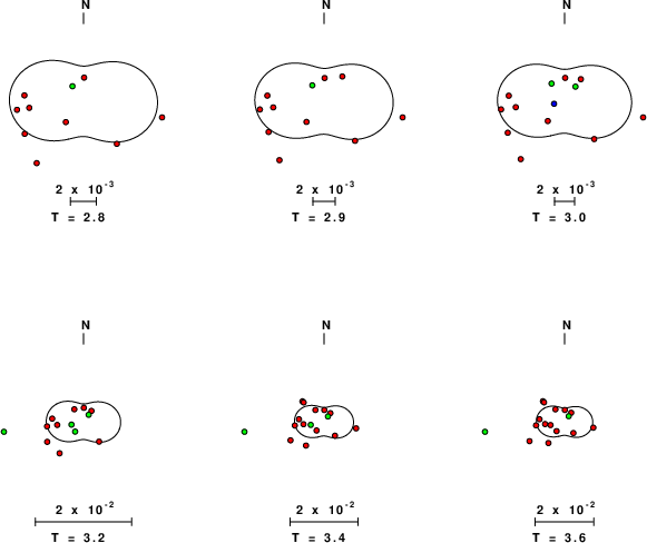
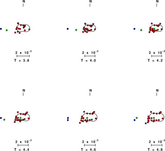
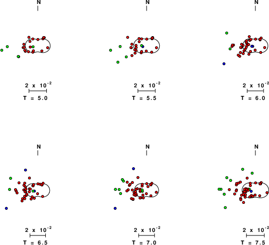
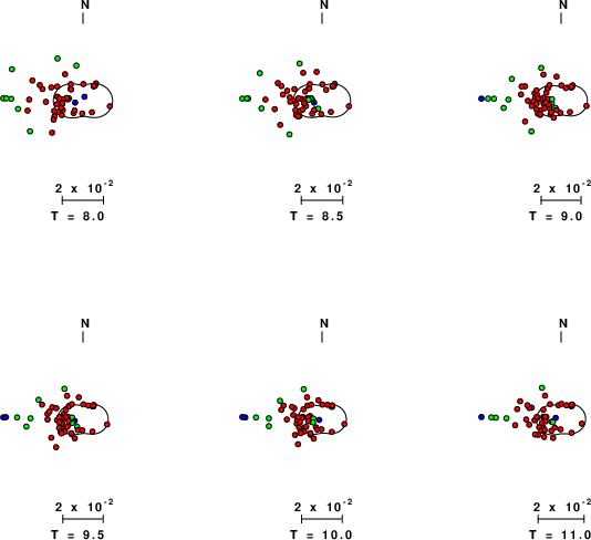
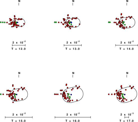
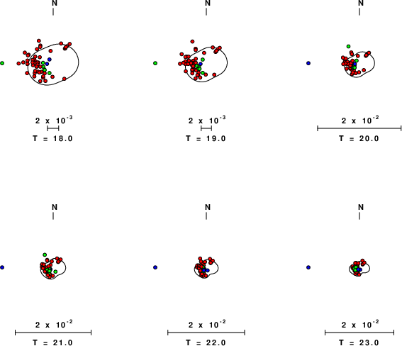
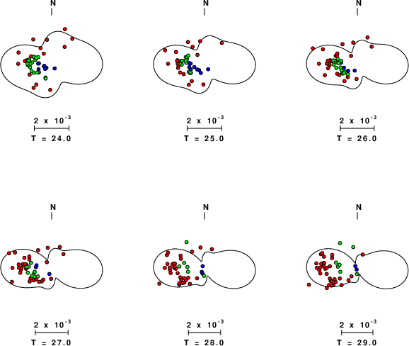
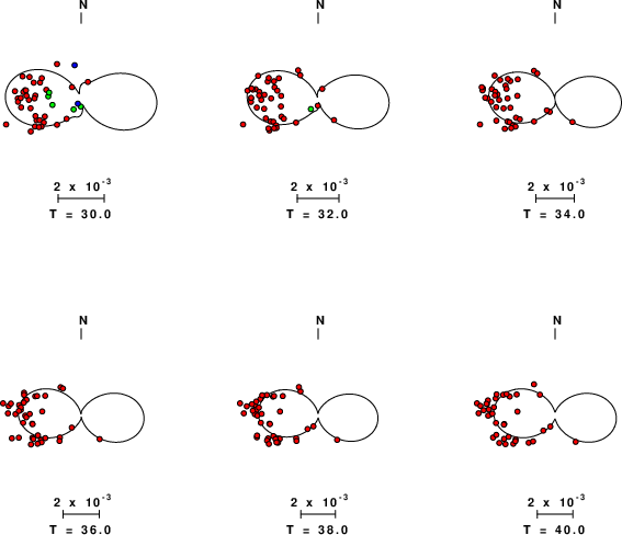
| Focal mechanism sensitivity at the preferred depth. The red color indicates a very good fit to the waveforms. Each solution is plotted as a vector at a given value of strike and dip with the angle of the vector representing the rake angle, measured, with respect to the upward vertical (N) in the figure. |
A check on the assumed source location is possible by looking at the time shifts between the observed and predicted traces. The time shifts for waveform matching arise for several reasons:
Time_shift = A + B cos Azimuth + C Sin Azimuth
The time shifts for this inversion lead to the next figure:
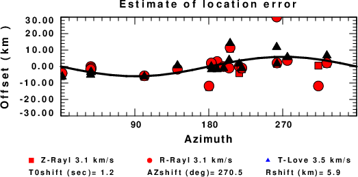
The derived shift in origin time and epicentral coordinates are given at the bottom of the figure.
The following figure shows the stations used in the grid search for the best focal mechanism to fit the surface-wave spectral amplitudes of the Love and Rayleigh waves.
|
|
|
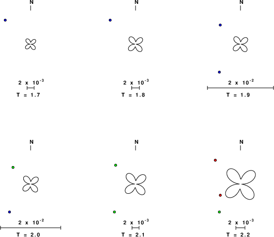
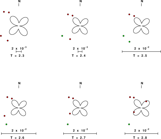
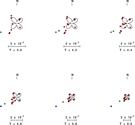
The surface-wave determined focal mechanism is shown here.
  NODAL PLANES


  STK=     179.99
  DIP=      55.00
 RAKE=      85.00

             OR

  STK=       8.66
  DIP=      35.32
 RAKE=      97.10


DEPTH = 10.0 km

Mw = 4.96
Best Fit 0.8355 - P-T axis plot gives solutions with FIT greater than FIT90
 |
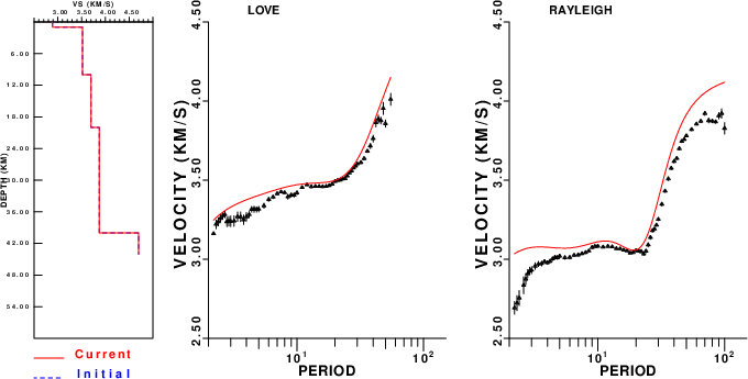
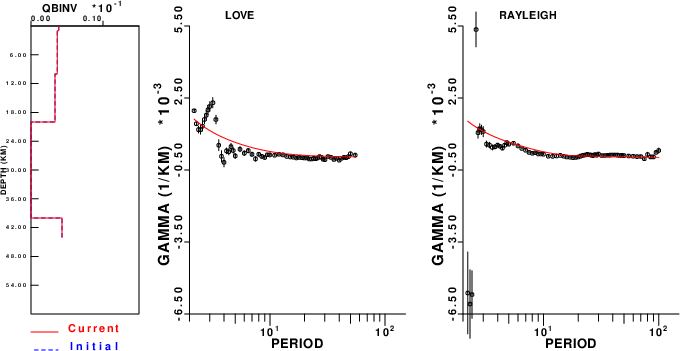
Surface wave analysis was performed using codes from Computer Programs in Seismology, specifically the multiple filter analysis program do_mft and the surface-wave radiation pattern search program srfgrd96.
Digital data were collected, instrument response removed and traces converted
to Z, R an T components. Multiple filter analysis was applied to the Z and T traces to obtain the Rayleigh- and Love-wave spectral amplitudes, respectively.
These were input to the search program which examined all depths between 1 and 25 km
and all possible mechanisms.
|
|
|

|
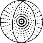
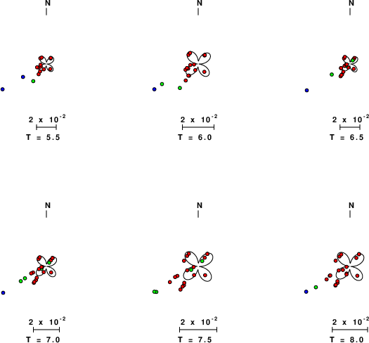
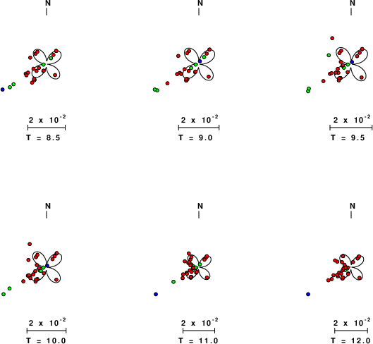
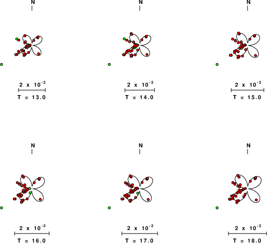
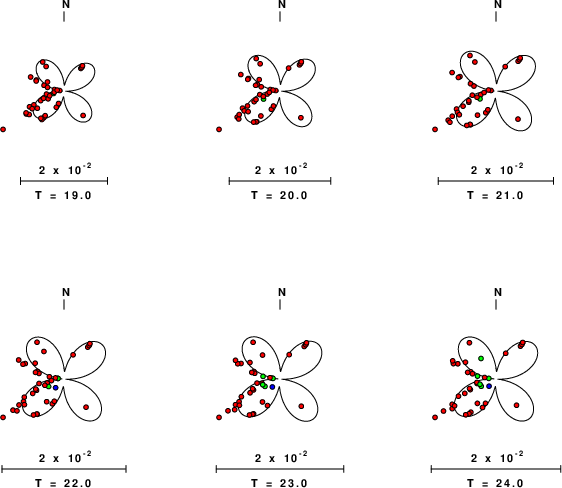
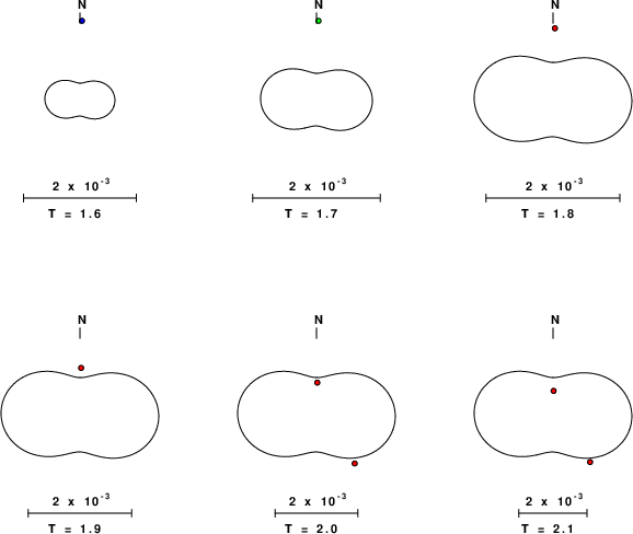
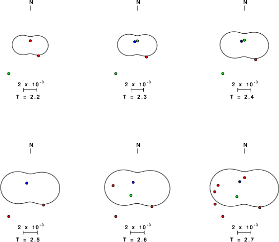
| Pressure-tension axis trends. Since the surface-wave spectra search does not distinguish between P and T axes and since there is a 180 ambiguity in strike, all possible P and T axes are plotted. First motion data and waveforms will be used to select the preferred mechanism. The purpose of this plot is to provide an idea of the possible range of solutions. The P and T-axes for all mechanisms with goodness of fit greater than 0.9 FITMAX (above) are plotted here. |
|
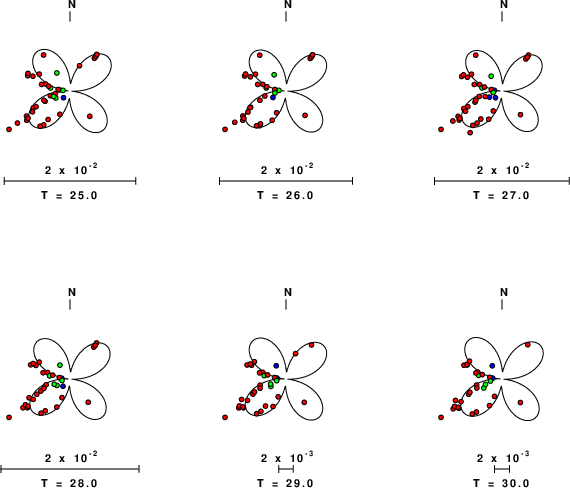
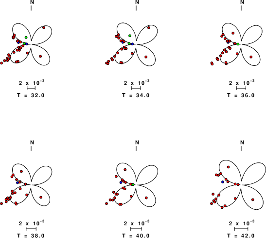
| Focal mechanism sensitivity at the preferred depth. The red color indicates a very good fit to the Love and Rayleigh wave radiation patterns. Each solution is plotted as a vector at a given value of strike and dip with the angle of the vector representing the rake angle, measured, with respect to the upward vertical (N) in the figure. Because of the symmetry of the spectral amplitude rediation patterns, only strikes from 0-180 degrees are sampled. |
|
|
The CUS.model used for the waveform synthetic seismograms and for the surface wave eigenfunctions and dispersion is as follows (The format is in the model96 format of Computer Programs in Seismology).
MODEL.01
CUS Model with Q from simple gamma values
ISOTROPIC
KGS
FLAT EARTH
1-D
CONSTANT VELOCITY
LINE08
LINE09
LINE10
LINE11
  H(KM) VP(KM/S) VS(KM/S) RHO(GM/CC)   QP   QS  ETAP  ETAS  FREFP  FREFS
  1.0000  5.0000  2.8900  2.5000 0.172E-02 0.387E-02 0.00  0.00  1.00  1.00
  9.0000  6.1000  3.5200  2.7300 0.160E-02 0.363E-02 0.00  0.00  1.00  1.00
 10.0000  6.4000  3.7000  2.8200 0.149E-02 0.336E-02 0.00  0.00  1.00  1.00
 20.0000  6.7000  3.8700  2.9020 0.000E-04 0.000E-04 0.00  0.00  1.00  1.00
  0.0000  8.1500  4.7000  3.3640 0.194E-02 0.431E-02 0.00  0.00  1.00  1.00