Location

Location ANSS

The ANSS event ID is uw10474303 and the event page is at https://earthquake.usgs.gov/earthquakes/eventpage/uw10474303/executive.

1999/07/03 01:43:54 47.074 -123.464 40.0 5.8 Washington

Focal Mechanism

USGS/SLU Moment Tensor Solution ENS 1999/07/03 01:43:54:0 47.07 -123.46 40.0 5.8 Washington Stations used: BK.CMB US.AHID US.ELK US.HAWA US.MNV US.NEW US.WVOR UU.CTU UU.HVU UU.NOQ UW.LON UW.LTY Filtering commands used: cut o DIST/3.3 -40 o DIST/3.3 +50 rtr taper w 0.1 hp c 0.03 n 3 lp c 0.07 n 3 Best Fitting Double Couple Mo = 4.47e+24 dyne-cm Mw = 5.70 Z = 44 km Plane Strike Dip Rake NP1 165 50 -95 NP2 353 40 -84 Principal Axes: Axis Value Plunge Azimuth T 4.47e+24 5 259 N 0.00e+00 4 168 P -4.47e+24 84 40 Moment Tensor: (dyne-cm) Component Value Mxx 1.44e+23 Mxy 8.37e+23 Mxz -4.42e+23 Myy 4.24e+24 Myz -6.82e+23 Mzz -4.38e+24 #------####### ####----------######## ######--------------######## ######----------------######## #######-------------------######## ########--------------------######## ########---------------------######### #########----------------------######### #########------------ --------######## ##########------------ P --------######### ###########----------- --------######### ###########----------------------######### ########----------------------######### T #########---------------------######## ##########--------------------######## ###########--------------------####### ###########------------------####### ############---------------####### ###########-------------###### ############----------###### ###########------##### ############## Global CMT Convention Moment Tensor: R T P -4.38e+24 -4.42e+23 6.82e+23 -4.42e+23 1.44e+23 -8.37e+23 6.82e+23 -8.37e+23 4.24e+24 Details of the solution is found at http://www.eas.slu.edu/eqc/eqc_mt/MECH.NA/19990703014354/index.html

Preferred Solution

The preferred solution from an analysis of the surface-wave spectral amplitude radiation pattern, waveform inversion or first motion observations is

      STK = 165
      DIP = 50
     RAKE = -95
       MW = 5.70
       HS = 44.0

The NDK file is 19990703014354.ndk The waveform inversion is preferred.

Moment Tensor Comparison

The following compares this source inversion to those provided by others. The purpose is to look for major differences and also to note slight differences that might be inherent to the processing procedure. For completeness the USGS/SLU solution is repeated from above.

SLU GCMT

USGS/SLU Moment Tensor Solution ENS 1999/07/03 01:43:54:0 47.07 -123.46 40.0 5.8 Washington Stations used: BK.CMB US.AHID US.ELK US.HAWA US.MNV US.NEW US.WVOR UU.CTU UU.HVU UU.NOQ UW.LON UW.LTY Filtering commands used: cut o DIST/3.3 -40 o DIST/3.3 +50 rtr taper w 0.1 hp c 0.03 n 3 lp c 0.07 n 3 Best Fitting Double Couple Mo = 4.47e+24 dyne-cm Mw = 5.70 Z = 44 km Plane Strike Dip Rake NP1 165 50 -95 NP2 353 40 -84 Principal Axes: Axis Value Plunge Azimuth T 4.47e+24 5 259 N 0.00e+00 4 168 P -4.47e+24 84 40 Moment Tensor: (dyne-cm) Component Value Mxx 1.44e+23 Mxy 8.37e+23 Mxz -4.42e+23 Myy 4.24e+24 Myz -6.82e+23 Mzz -4.38e+24 #------####### ####----------######## ######--------------######## ######----------------######## #######-------------------######## ########--------------------######## ########---------------------######### #########----------------------######### #########------------ --------######## ##########------------ P --------######### ###########----------- --------######### ###########----------------------######### ########----------------------######### T #########---------------------######## ##########--------------------######## ###########--------------------####### ###########------------------####### ############---------------####### ###########-------------###### ############----------###### ###########------##### ############## Global CMT Convention Moment Tensor: R T P -4.38e+24 -4.42e+23 6.82e+23 -4.42e+23 1.44e+23 -8.37e+23 6.82e+23 -8.37e+23 4.24e+24 Details of the solution is found at http://www.eas.slu.edu/eqc/eqc_mt/MECH.NA/19990703014354/index.html

Global CMT Best Fitting Double Couple Mo = 5.62e+24 dyne-cm Mw = 5.80 Z = 45 km Plane Strike Dip Rake NP1 345 61 -108 NP2 199 34 -61 Principal Axes: Axis Value Plunge Azimuth T 5.62e+24 14 88 N 0.00e+00 16 354 P -5.62e+24 69 218 Moment Tensor: (dyne-cm) Component Value Mxx -4.55e+23 Mxy -2.02e+23 Mxz 1.54e+24 Myy 5.02e+24 Myz 2.48e+24 Mzz -4.56e+24 ###--------### ###################### #########-----############## ########---------############# ########------------############## ########--------------############## ########----------------############## ########------------------############## #######-------------------############## #######---------------------########## # #######---------------------########## T # #######----------------------######### # #######--------- ----------############# ######--------- P ----------############ ######--------- ----------############ #####----------------------########### #####---------------------########## ####---------------------######### ###--------------------####### ###------------------####### ##----------------#### -------------# Harvard Convention Moment Tensor: R T F -4.56e+24 1.54e+24 -2.48e+24 1.54e+24 -4.55e+23 2.02e+23 -2.48e+24 2.02e+23 5.02e+24

Context

The left panel of the next figure presents the focal mechanism for this earthquake (red) in the context of other nearby events (blue) in the SLU Moment Tensor Catalog. The right panel shows the inferred direction of maximum compressive stress and the type of faulting (green is strike-slip, red is normal, blue is thrust; oblique is shown by a combination of colors). Thus context plot is useful for assessing the appropriateness of the moment tensor of this event.

Waveform Inversion using wvfgrd96

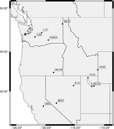
The focal mechanism was determined using broadband seismic waveforms. The location of the event (star) and the stations used for (red) the waveform inversion are shown in the next figure.

Location of broadband stations used for waveform inversion

The program wvfgrd96 was used with good traces observed at short distance to determine the focal mechanism, depth and seismic moment. This technique requires a high quality signal and well determined velocity model for the Green's functions. To the extent that these are the quality data, this type of mechanism should be preferred over the radiation pattern technique which requires the separate step of defining the pressure and tension quadrants and the correct strike.

The observed and predicted traces are filtered using the following gsac commands:

cut o DIST/3.3 -40 o DIST/3.3 +50
rtr
taper w 0.1
hp c 0.03 n 3 
lp c 0.07 n 3

The results of this grid search are as follow:

           DEPTH  STK   DIP  RAKE   MW    FIT
WVFGRD96    1.0   170    50    90   4.97 0.2900
WVFGRD96    2.0   345    40    85   5.07 0.3573
WVFGRD96    3.0    -5    40    85   5.17 0.4205
WVFGRD96    4.0   340    45    60   5.21 0.4050
WVFGRD96    5.0   325    60    25   5.21 0.3687
WVFGRD96    6.0   320    75     5   5.24 0.3529
WVFGRD96    7.0   320    80    -5   5.27 0.3407
WVFGRD96    8.0   320    90   -25   5.30 0.3337
WVFGRD96    9.0   315    80   -20   5.28 0.3199
WVFGRD96   10.0   315    80   -25   5.29 0.3082
WVFGRD96   11.0   125    65   -40   5.27 0.3048
WVFGRD96   12.0   115    45   -25   5.22 0.3218
WVFGRD96   13.0   115    45   -25   5.24 0.3384
WVFGRD96   14.0   105    40   -20   5.21 0.3541
WVFGRD96   15.0   105    40   -20   5.22 0.3693
WVFGRD96   16.0   100    35   -10   5.21 0.3836
WVFGRD96   17.0   100    35    -5   5.23 0.3972
WVFGRD96   18.0   100    35    -5   5.24 0.4099
WVFGRD96   19.0    55    60    35   5.39 0.4286
WVFGRD96   20.0    55    60    35   5.40 0.4454
WVFGRD96   21.0    55    55    30   5.44 0.4620
WVFGRD96   22.0    55    55    35   5.45 0.4780
WVFGRD96   23.0    55    55    35   5.46 0.4933
WVFGRD96   24.0    55    55    35   5.48 0.5079
WVFGRD96   25.0    55    55    35   5.49 0.5217
WVFGRD96   26.0    55    55    35   5.50 0.5346
WVFGRD96   27.0    60    55    45   5.51 0.5474
WVFGRD96   28.0   355    50   -70   5.42 0.5609
WVFGRD96   29.0     0    50   -65   5.44 0.5846
WVFGRD96   30.0    -5    45   -70   5.45 0.6084
WVFGRD96   31.0    -5    45   -70   5.46 0.6307
WVFGRD96   32.0     0    45   -65   5.48 0.6502
WVFGRD96   33.0     0    45   -70   5.48 0.6660
WVFGRD96   34.0   355    45   -75   5.49 0.6798
WVFGRD96   35.0   355    45   -75   5.51 0.6899
WVFGRD96   36.0   340    45   -90   5.52 0.6980
WVFGRD96   37.0   345    40   -80   5.54 0.7054
WVFGRD96   38.0   345    40   -80   5.56 0.7134
WVFGRD96   39.0   345    40   -80   5.58 0.7218
WVFGRD96   40.0   355    40   -80   5.66 0.7036
WVFGRD96   41.0   355    40   -80   5.67 0.7181
WVFGRD96   42.0   350    40   -85   5.68 0.7277
WVFGRD96   43.0   350    40   -85   5.69 0.7326
WVFGRD96   44.0   165    50   -95   5.70 0.7339
WVFGRD96   45.0   165    50   -95   5.71 0.7319
WVFGRD96   46.0   170    50   -85   5.72 0.7292
WVFGRD96   47.0   170    50   -85   5.72 0.7248
WVFGRD96   48.0   345    40   -95   5.73 0.7179
WVFGRD96   49.0   340    40  -100   5.73 0.7108
WVFGRD96   50.0   170    50   -85   5.74 0.7021
WVFGRD96   51.0   160    55  -100   5.75 0.6928
WVFGRD96   52.0   160    55   -95   5.75 0.6840
WVFGRD96   53.0   160    55   -95   5.76 0.6742
WVFGRD96   54.0   160    55   -95   5.76 0.6629
WVFGRD96   55.0   165    55   -90   5.76 0.6519
WVFGRD96   56.0   345    35   -90   5.77 0.6402
WVFGRD96   57.0   345    35   -90   5.77 0.6277
WVFGRD96   58.0   340    35   -95   5.77 0.6144
WVFGRD96   59.0   340    35  -100   5.77 0.6018

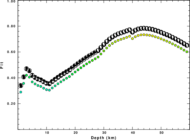
The best solution is

WVFGRD96   44.0   165    50   -95   5.70 0.7339

The mechanism corresponding to the best fit is

Figure 1. Waveform inversion focal mechanism

The best fit as a function of depth is given in the following figure:

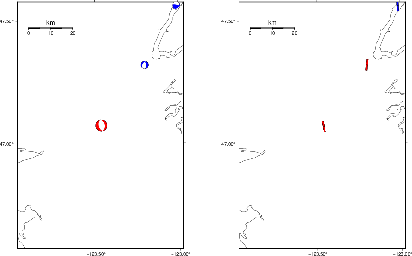
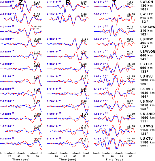
Figure 2. Depth sensitivity for waveform mechanism

The comparison of the observed and predicted waveforms is given in the next figure. The red traces are the observed and the blue are the predicted. Each observed-predicted component is plotted to the same scale and peak amplitudes are indicated by the numbers to the left of each trace. A pair of numbers is given in black at the right of each predicted traces. The upper number it the time shift required for maximum correlation between the observed and predicted traces. This time shift is required because the synthetics are not computed at exactly the same distance as the observed, the velocity model used in the predictions may not be perfect and the epicentral parameters may be be off. A positive time shift indicates that the prediction is too fast and should be delayed to match the observed trace (shift to the right in this figure). A negative value indicates that the prediction is too slow. The lower number gives the percentage of variance reduction to characterize the individual goodness of fit (100% indicates a perfect fit).

The bandpass filter used in the processing and for the display was

cut o DIST/3.3 -40 o DIST/3.3 +50
rtr
taper w 0.1
hp c 0.03 n 3 
lp c 0.07 n 3

Figure 3. Waveform comparison for selected depth. Red: observed; Blue - predicted. The time shift with respect to the model prediction is indicated. The percent of fit is also indicated. The time scale is relative to the first trace sample.

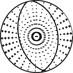
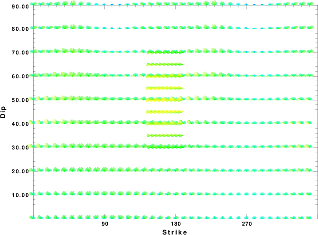
Focal mechanism sensitivity at the preferred depth. The red color indicates a very good fit to the waveforms. Each solution is plotted as a vector at a given value of strike and dip with the angle of the vector representing the rake angle, measured, with respect to the upward vertical (N) in the figure.

A check on the assumed source location is possible by looking at the time shifts between the observed and predicted traces. The time shifts for waveform matching arise for several reasons:

The origin time and epicentral distance are incorrect
The velocity model used for the inversion is incorrect
The velocity model used to define the P-arrival time is not the same as the velocity model used for the waveform inversion (assuming that the initial trace alignment is based on the P arrival time)

Assuming only a mislocation, the time shifts are fit to a functional form:

 Time_shift = A + B cos Azimuth + C Sin Azimuth

The time shifts for this inversion lead to the next figure:

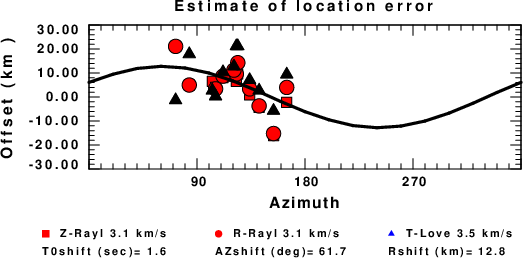
The derived shift in origin time and epicentral coordinates are given at the bottom of the figure.

Velocity Model

The WUS.model used for the waveform synthetic seismograms and for the surface wave eigenfunctions and dispersion is as follows (The format is in the model96 format of Computer Programs in Seismology).

MODEL.01
Model after     8 iterations
ISOTROPIC
KGS
FLAT EARTH
1-D
CONSTANT VELOCITY
LINE08
LINE09
LINE10
LINE11
      H(KM)   VP(KM/S)   VS(KM/S) RHO(GM/CC)         QP         QS       ETAP       ETAS      FREFP      FREFS
     1.9000     3.4065     2.0089     2.2150  0.302E-02  0.679E-02   0.00       0.00       1.00       1.00    
     6.1000     5.5445     3.2953     2.6089  0.349E-02  0.784E-02   0.00       0.00       1.00       1.00    
    13.0000     6.2708     3.7396     2.7812  0.212E-02  0.476E-02   0.00       0.00       1.00       1.00    
    19.0000     6.4075     3.7680     2.8223  0.111E-02  0.249E-02   0.00       0.00       1.00       1.00    
     0.0000     7.9000     4.6200     3.2760  0.164E-10  0.370E-10   0.00       0.00       1.00       1.00

Last Changed Thu Apr 25 12:47:39 PM CDT 2024