Location

Location ANSS

The ANSS event ID is usp00089hq and the event page is at https://earthquake.usgs.gov/earthquakes/eventpage/usp00089hq/executive.

1997/10/24 08:35:17 31.118 -87.339 10.0 4.8 Alabama

Focal Mechanism

USGS/SLU Moment Tensor Solution ENS 1997/10/24 08:35:17:0 31.12 -87.34 10.0 4.8 Alabama Stations used: IU.CCM IU.SSPA IU.WCI NM.SLM US.AAM US.BLA US.CBKS US.CEH US.GOGA US.JFWS US.MCWV US.MIAR US.OXF US.WMOK Filtering commands used: cut o DIST/3.3 -40 o DIST/3.3 +50 rtr taper w 0.1 hp c 0.03 n 3 lp c 0.10 n 3 Best Fitting Double Couple Mo = 8.41e+22 dyne-cm Mw = 4.55 Z = 2 km Plane Strike Dip Rake NP1 285 50 -85 NP2 97 40 -96 Principal Axes: Axis Value Plunge Azimuth T 8.41e+22 5 11 N 0.00e+00 4 102 P -8.41e+22 84 230 Moment Tensor: (dyne-cm) Component Value Mxx 7.98e+22 Mxy 1.58e+22 Mxz 1.28e+22 Myy 2.72e+21 Myz 8.32e+21 Mzz -8.25e+22 ######### T ## ############# ###### ############################ ############################## ################################## #######------------################# ###-----------------------############ #-----------------------------########## ---------------------------------####### ------------------------------------###### #----------------- -----------------#### ##---------------- P ------------------### ###--------------- -------------------## ###------------------------------------# #####---------------------------------## #######---------------------------#### #########---------------------###### ##############---------########### ############################## ############################ ###################### ############## Global CMT Convention Moment Tensor: R T P -8.25e+22 1.28e+22 -8.32e+21 1.28e+22 7.98e+22 -1.58e+22 -8.32e+21 -1.58e+22 2.72e+21 Details of the solution is found at http://www.eas.slu.edu/eqc/eqc_mt/MECH.NA/19971024083517/index.html

Preferred Solution

      STK = 285
      DIP = 50
     RAKE = -85
       MW = 4.55
       HS = 2.0

The NDK file is 19971024083517.ndk The waveform inversion is preferred.

Context

Waveform Inversion using wvfgrd96

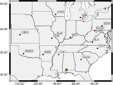
The focal mechanism was determined using broadband seismic waveforms. The location of the event (star) and the stations used for (red) the waveform inversion are shown in the next figure.

Location of broadband stations used for waveform inversion

The program wvfgrd96 was used with good traces observed at short distance to determine the focal mechanism, depth and seismic moment. This technique requires a high quality signal and well determined velocity model for the Green's functions. To the extent that these are the quality data, this type of mechanism should be preferred over the radiation pattern technique which requires the separate step of defining the pressure and tension quadrants and the correct strike.

The observed and predicted traces are filtered using the following gsac commands:

cut o DIST/3.3 -40 o DIST/3.3 +50
rtr
taper w 0.1
hp c 0.03 n 3 
lp c 0.10 n 3 

           DEPTH  STK   DIP  RAKE   MW    FIT
WVFGRD96    1.0   125    40   -50   4.45 0.2094
WVFGRD96    2.0   285    50   -85   4.55 0.2389
WVFGRD96    3.0    95    40   -95   4.61 0.2198
WVFGRD96    4.0   280    55   -80   4.55 0.1646
WVFGRD96    5.0    80    30  -110   4.47 0.1418
WVFGRD96    6.0   285    65   -75   4.44 0.1424
WVFGRD96    7.0   155    65    35   4.46 0.1501
WVFGRD96    8.0   155    65    35   4.47 0.1581
WVFGRD96    9.0   150    65    40   4.47 0.1652
WVFGRD96   10.0   155    60    40   4.51 0.1690
WVFGRD96   11.0   155    55    50   4.52 0.1753
WVFGRD96   12.0   155    55    50   4.53 0.1816
WVFGRD96   13.0   155    55    50   4.54 0.1870
WVFGRD96   14.0   155    55    50   4.55 0.1916
WVFGRD96   15.0    95    55    85   4.53 0.1960
WVFGRD96   16.0    95    55    85   4.54 0.2019
WVFGRD96   17.0    95    55    85   4.56 0.2073
WVFGRD96   18.0    95    55    85   4.57 0.2121
WVFGRD96   19.0    95    55    85   4.58 0.2164
WVFGRD96   20.0    95    55    85   4.62 0.2203
WVFGRD96   21.0    95    55    85   4.63 0.2234
WVFGRD96   22.0    95    55    90   4.64 0.2256
WVFGRD96   23.0   275    35    90   4.65 0.2273
WVFGRD96   24.0   275    35    90   4.66 0.2281
WVFGRD96   25.0   270    40    85   4.67 0.2284
WVFGRD96   26.0   270    40    85   4.68 0.2286
WVFGRD96   27.0   270    40    85   4.68 0.2282
WVFGRD96   28.0   100    50    95   4.69 0.2272
WVFGRD96   29.0   270    45    85   4.70 0.2260

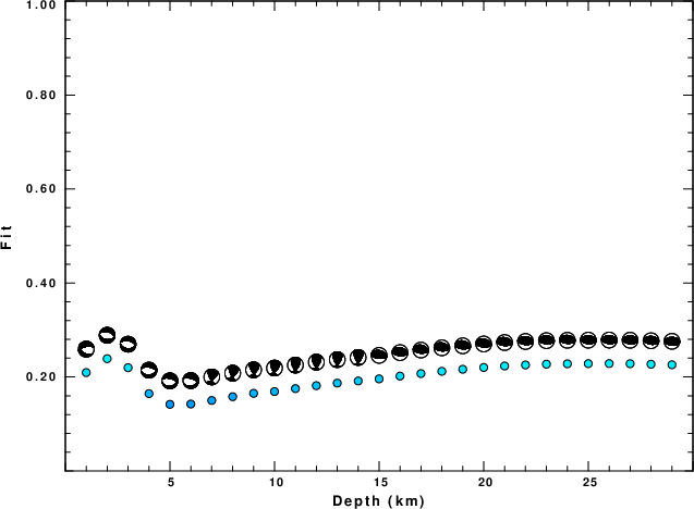
The best solution is

WVFGRD96    2.0   285    50   -85   4.55 0.2389

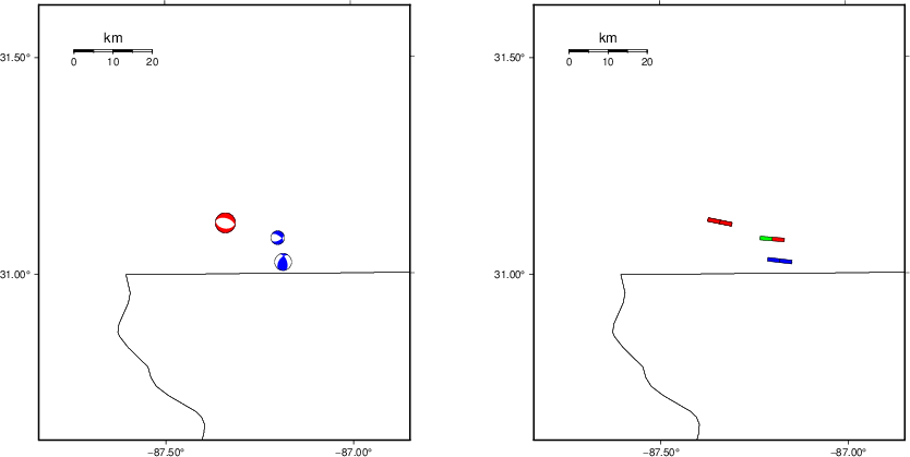
The mechanism corresponding to the best fit is

Figure 1. Waveform inversion focal mechanism

The best fit as a function of depth is given in the following figure:

Figure 2. Depth sensitivity for waveform mechanism

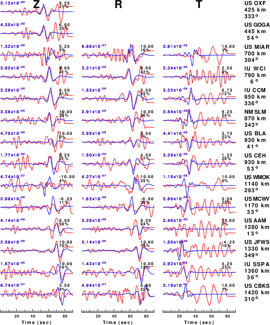
The comparison of the observed and predicted waveforms is given in the next figure. The red traces are the observed and the blue are the predicted. Each observed-predicted component is plotted to the same scale and peak amplitudes are indicated by the numbers to the left of each trace. A pair of numbers is given in black at the right of each predicted traces. The upper number it the time shift required for maximum correlation between the observed and predicted traces. This time shift is required because the synthetics are not computed at exactly the same distance as the observed, the velocity model used in the predictions may not be perfect and the epicentral parameters may be be off. A positive time shift indicates that the prediction is too fast and should be delayed to match the observed trace (shift to the right in this figure). A negative value indicates that the prediction is too slow. The lower number gives the percentage of variance reduction to characterize the individual goodness of fit (100% indicates a perfect fit).

The bandpass filter used in the processing and for the display was

cut o DIST/3.3 -40 o DIST/3.3 +50
rtr
taper w 0.1
hp c 0.03 n 3 
lp c 0.10 n 3 

Figure 3. Waveform comparison for selected depth. Red: observed; Blue - predicted. The time shift with respect to the model prediction is indicated. The percent of fit is also indicated. The time scale is relative to the first trace sample.

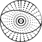
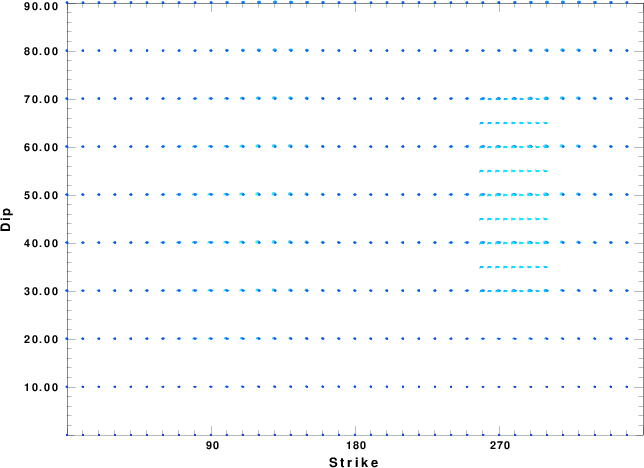
Focal mechanism sensitivity at the preferred depth. The red color indicates a very good fit to the waveforms. Each solution is plotted as a vector at a given value of strike and dip with the angle of the vector representing the rake angle, measured, with respect to the upward vertical (N) in the figure.

A check on the assumed source location is possible by looking at the time shifts between the observed and predicted traces. The time shifts for waveform matching arise for several reasons:

• The origin time and epicentral distance are incorrect
• The velocity model used for the inversion is incorrect
• The velocity model used to define the P-arrival time is not the same as the velocity model used for the waveform inversion (assuming that the initial trace alignment is based on the P arrival time)

 Time_shift = A + B cos Azimuth + C Sin Azimuth

The time shifts for this inversion lead to the next figure:

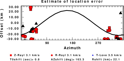
The derived shift in origin time and epicentral coordinates are given at the bottom of the figure.

Velocity Model

The CUS.model used for the waveform synthetic seismograms and for the surface wave eigenfunctions and dispersion is as follows (The format is in the model96 format of Computer Programs in Seismology).

MODEL.01
CUS Model with Q from simple gamma values
ISOTROPIC
KGS
FLAT EARTH
1-D
CONSTANT VELOCITY
LINE08
LINE09
LINE10
LINE11
  H(KM) VP(KM/S) VS(KM/S) RHO(GM/CC)   QP   QS  ETAP  ETAS  FREFP  FREFS
  1.0000  5.0000  2.8900  2.5000 0.172E-02 0.387E-02 0.00  0.00  1.00  1.00 
  9.0000  6.1000  3.5200  2.7300 0.160E-02 0.363E-02 0.00  0.00  1.00  1.00 
 10.0000  6.4000  3.7000  2.8200 0.149E-02 0.336E-02 0.00  0.00  1.00  1.00 
 20.0000  6.7000  3.8700  2.9020 0.000E-04 0.000E-04 0.00  0.00  1.00  1.00 
  0.0000  8.1500  4.7000  3.3640 0.194E-02 0.431E-02 0.00  0.00  1.00  1.00