
2008/11/20 19:23:01 32.3590 -115.3550 10.0 5.00 Baja California, Mexico
USGS Felt map for this earthquake
USGS Felt reports page for California
 SLU Moment Tensor Solution
 2008/11/20 19:23:01  32.3590  -115.3550  10.0  5.00 Baja California, Mexico

 Best Fitting Double Couple
    Mo = 1.19e+23 dyne-cm
    Mw = 4.65
    Z  = 14 km
     Plane   Strike  Dip  Rake
      NP1      145    76   159
      NP2      240    70    15
 Principal Axes:
   Axis    Value   Plunge  Azimuth
     T   1.19e+23     24     101
     N   0.00e+00     65     292
     P  -1.19e+23      4     193


 Moment Tensor: (dyne-cm)
    Component  Value
       Mxx    -1.08e+23
       Mxy    -4.54e+22
       Mxz    -7.75e+20
       Myy     8.85e+22
       Myz     4.58e+22
       Mzz     1.98e+22


                     --------------
                 ----------------------
              ##--------------------------
             ####--------------------------
           ######----------------------------
          ########-----------------------#####
         ##########---------------#############
        ############---------###################
        #############-----######################
       ###############-##########################
       #############---##########################
       ###########------##################   ####
       #########----------################ T ####
        ######-------------###############   ###
        ####----------------####################
         ##-------------------#################
          ----------------------##############
           ----------------------############
             -----------------------#######
              ------------------------####
                 -----   --------------
                     - P ----------


 Harvard Convention
 Moment Tensor:
      R          T          F
  1.98e+22  -7.75e+20  -4.58e+22
 -7.75e+20  -1.08e+23   4.54e+22
 -4.58e+22   4.54e+22   8.85e+22


Details of the solution is found at

http://www.eas.slu.edu/eqc/eqc_mt/MECH.NA/20081120192301/index.html
|
      STK = 240
      DIP = 70
     RAKE = 15
       MW = 4.65
       HS = 14.0
The waveform inversion is preferred. The surface wave solution was biased by the large number of observations at 1000-2000 km. Using the more appropriate WUS model gives a different weight to these observations at short period because of the disparity between the observed and predicted amplitudes. The use of the CUS model is for the purpose of testing the soltuion and not for the determination of the gamma coefficient for anelastic attenuation.
The following compares this source inversion to others
 SLU Moment Tensor Solution
 2008/11/20 19:23:01  32.3590  -115.3550  10.0  5.00 Baja California, Mexico

 Best Fitting Double Couple
    Mo = 1.19e+23 dyne-cm
    Mw = 4.65
    Z  = 14 km
     Plane   Strike  Dip  Rake
      NP1      145    76   159
      NP2      240    70    15
 Principal Axes:
   Axis    Value   Plunge  Azimuth
     T   1.19e+23     24     101
     N   0.00e+00     65     292
     P  -1.19e+23      4     193


 Moment Tensor: (dyne-cm)
    Component  Value
       Mxx    -1.08e+23
       Mxy    -4.54e+22
       Mxz    -7.75e+20
       Myy     8.85e+22
       Myz     4.58e+22
       Mzz     1.98e+22


                     --------------
                 ----------------------
              ##--------------------------
             ####--------------------------
           ######----------------------------
          ########-----------------------#####
         ##########---------------#############
        ############---------###################
        #############-----######################
       ###############-##########################
       #############---##########################
       ###########------##################   ####
       #########----------################ T ####
        ######-------------###############   ###
        ####----------------####################
         ##-------------------#################
          ----------------------##############
           ----------------------############
             -----------------------#######
              ------------------------####
                 -----   --------------
                     - P ----------


 Harvard Convention
 Moment Tensor:
      R          T          F
  1.98e+22  -7.75e+20  -4.58e+22
 -7.75e+20  -1.08e+23   4.54e+22
 -4.58e+22   4.54e+22   8.85e+22


Details of the solution is found at

http://www.eas.slu.edu/eqc/eqc_mt/MECH.NA/20081120192301/index.html
|
** SCSN Moment Tensor Solution Message **

REAL-TIME SOLUTION: NOT REVIEWED
Inversion Method: Complete Waveform
Number of Stations used: 6
Stations: CI.GLA CI.SDR CI.JEM CI.BOR CI.CTC CI.RXH

Real-Time Solution:
-------------------
Event ID    : 14404512
Magnitude   : 5.00
Depth (km)  : 37.1
Origin Time :  11/20/2008 19:23:01:900
Latitude    : 32.39
Longitude   : -115.32
Further Information at: http://pasadena.wr.usgs.gov/recenteqs/Quakes/ci14404512.htm

SCSN Moment Tensor Solution:
----------------------------
Moment Magnitude     : 4.67
Depth (km)           : 5
Variance Reduction(%): 92.03
Quality Factor       : A
   (A : Mw, MT good enough for distribution)
   (B : Mw only good enough for distribution)
   (C : Solution needs review before distribution)


Best Fitting Double Couple and CLVD Solution:
---------------------------------------------------

Moment Tensor: Scale = 10**21 Dyne-cm
    Component   Value
       Mxx      -95.4
       Mxy      -56.1
       Mxz      -10.2
       Myy      125
       Myz      -28.8
       Mzz      -29.9

Best Fitting Double Couple Solution:
--------------------------------------------------
 Moment Tensor: Scale = 10**23 Dyne-cm
    Component   Value
       Mxx     -1.085
       Mxy     -0.570
       Mxz     -0.195
       Myy      1.106
       Myz     -0.241
       Mzz     -0.021

 Principle Axes:
    Axis    Value   Plunge   Azimuth
      T     1.274       8      283
      N     0.000      76      157
      P    -1.274      11       15

 Best Fitting Double-Couple:
    Mo = 1.27E+23 Dyne-cm
    Plane   Strike   Rake   Dip
     NP1      149    -166    88
     NP2       59      -2    76

 Moment Magnitude = 4.67


                    -------
              -------------   ---
           ##-------------- P ------
         #####-------------   --------
       ########-------------------------
      ##########-------------------------
     #############----------------------##
    ###############-------------------#####
       #############----------------#######
   # T ##############-------------##########
   #   ###############----------############
   ####################------###############
   #####################---#################
   #####################-###################
    ################------#################
    ############-----------################
     #######-----------------#############
      ------------------------###########
       ------------------------#########
         -----------------------######
           ----------------------###
              -------------------
                    -------

     Lower Hemisphere Equiangle Projection

=============  Station Information ==============

Name       Distance     Azimuth     VR      ZCore
-------------------------------------------------
CI.GLA       86.684     32.080   93.107     13.00
CI.SDR      157.091    284.552   86.771     22.00
CI.JEM      142.146    302.955   91.111     18.00
CI.BOR      141.536    313.763   95.118     18.00
CI.CTC      153.615    336.133   90.594     19.00
CI.RXH       92.393    342.218   92.661     11.00
|
The focal mechanism was determined using broadband seismic waveforms. The location of the event and the and stations used for the waveform inversion are shown in the next figure.
|
|
|
|
The program wvfgrd96 was used with good traces observed at short distance to determine the focal mechanism, depth and seismic moment. This technique requires a high quality signal and well determined velocity model for the Green functions. To the extent that these are the quality data, this type of mechanism should be preferred over the radiation pattern technique which requires the separate step of defining the pressure and tension quadrants and the correct strike.
The observed and predicted traces are filtered using the following gsac commands:
hp c 0.02 n 3
lp c 0.05 n 3
The results of this grid search from 0.5 to 19 km depth are as follow:
           DEPTH  STK   DIP  RAKE   MW    FIT
WVFGRD96    0.5   235    75   -15   4.32 0.2822
WVFGRD96    1.0    55    80   -10   4.34 0.3027
WVFGRD96    2.0   235    75   -10   4.42 0.3738
WVFGRD96    3.0   235    75   -15   4.47 0.4053
WVFGRD96    4.0   235    75   -15   4.50 0.4247
WVFGRD96    5.0   235    75   -10   4.52 0.4386
WVFGRD96    6.0   235    75   -10   4.54 0.4503
WVFGRD96    7.0   235    75   -10   4.56 0.4616
WVFGRD96    8.0   235    70   -10   4.59 0.4743
WVFGRD96    9.0   235    70     5   4.60 0.4764
WVFGRD96   10.0   240    70    15   4.62 0.4815
WVFGRD96   11.0   240    70    15   4.63 0.4865
WVFGRD96   12.0   240    70    15   4.64 0.4906
WVFGRD96   13.0   240    70    15   4.65 0.4943
WVFGRD96   14.0   240    70    15   4.65 0.4963
WVFGRD96   15.0   240    70    15   4.66 0.4959
WVFGRD96   16.0   235    75    15   4.67 0.4960
WVFGRD96   17.0   235    75    15   4.68 0.4948
WVFGRD96   18.0    60    70    15   4.69 0.4916
WVFGRD96   19.0    55    70    10   4.69 0.4907
WVFGRD96   20.0    55    75    15   4.70 0.4891
WVFGRD96   21.0    55    75    15   4.71 0.4869
WVFGRD96   22.0    55    75   -15   4.72 0.4872
WVFGRD96   23.0    55    75   -15   4.73 0.4844
WVFGRD96   24.0    55    75   -15   4.74 0.4808
WVFGRD96   25.0    55    80   -15   4.74 0.4767
WVFGRD96   26.0    55    80   -15   4.75 0.4719
WVFGRD96   27.0    55    80   -15   4.76 0.4665
WVFGRD96   28.0    55    80   -15   4.76 0.4605
WVFGRD96   29.0    55    80   -15   4.77 0.4539
The best solution is
WVFGRD96 14.0 240 70 15 4.65 0.4963
The mechanism correspond to the best fit is

|
|
|
The best fit as a function of depth is given in the following figure:

|
|
|
The comparison of the observed and predicted waveforms is given in the next figure. The red traces are the observed and the blue are the predicted. Each observed-predicted componnet is plotted to the same scale and peak amplitudes are indicated by the numbers to the left of each trace. The number in black at the rightr of each predicted traces it the time shift required for maximum correlation between the observed and predicted traces. This time shift is required because the synthetics are not computed at exactly the same distance as the observed and because the velocity model used in the predictions may not be perfect. A positive time shift indicates that the prediction is too fast and should be delayed to match the observed trace (shift to the right in this figure). A negative value indicates that the prediction is too slow. The bandpass filter used in the processing and for the display was
hp c 0.02 n 3
lp c 0.05 n 3

|
|
|

|
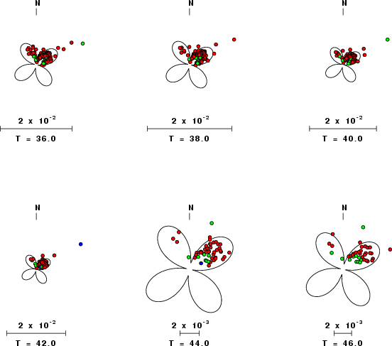
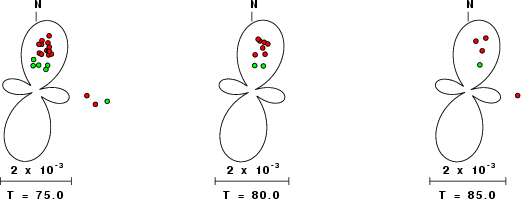
| Focal mechanism sensitivity at the preferred depth. The red color indicates a very good fit to thewavefroms. Each solution is plotted as a vector at a given value of strike and dip with the angle of the vector representing the rake angle, measured, with respect to the upward vertical (N) in the figure. |
The following figure shows the stations used in the grid search for the best focal mechanism to fit the surface-wave spectral amplitudes of the Love and Rayleigh waves.

|
|
|
The surface-wave determined focal mechanism is shown here.
  NODAL PLANES


  STK=     244.99
  DIP=      70.00
 RAKE=      39.99

             OR

  STK=     138.98
  DIP=      52.85
 RAKE=     154.58


DEPTH = 11.0 km

Mw = 4.84
Best Fit 0.8660 - P-T axis plot gives solutions with FIT greater than FIT90
 |
The P-wave first motion data for focal mechanism studies are as follow:
Sta Az Dist First motion
Surface wave analysis was performed using codes from Computer Programs in Seismology, specifically the multiple filter analysis program do_mft and the surface-wave radiation pattern search program srfgrd96.
Digital data were collected, instrument response removed and traces converted
to Z, R an T components. Multiple filter analysis was applied to the Z and T traces to obtain the Rayleigh- and Love-wave spectral amplitudes, respectively.
These were input to the search program which examined all depths between 1 and 25 km
and all possible mechanisms.

|
|
|

|
| Pressure-tension axis trends. Since the surface-wave spectra search does not distinguish between P and T axes and since there is a 180 ambiguity in strike, all possible P and T axes are plotted. First motion data and waveforms will be used to select the preferred mechanism. The purpose of this plot is to provide an idea of the possible range of solutions. The P and T-axes for all mechanisms with goodness of fit greater than 0.9 FITMAX (above) are plotted here. |

|
| Focal mechanism sensitivity at the preferred depth. The red color indicates a very good fit to the Love and Rayleigh wave radiation patterns. Each solution is plotted as a vector at a given value of strike and dip with the angle of the vector representing the rake angle, measured, with respect to the upward vertical (N) in the figure. Because of the symmetry of the spectral amplitude rediation patterns, only strikes from 0-180 degrees are sampled. |
The distribution of broadband stations with azimuth and distance is
Listing of broadband stations used
Since the analysis of the surface-wave radiation patterns uses only spectral amplitudes and because the surfave-wave radiation patterns have a 180 degree symmetry, each surface-wave solution consists of four possible focal mechanisms corresponding to the interchange of the P- and T-axes and a roation of the mechanism by 180 degrees. To select one mechanism, P-wave first motion can be used. This was not possible in this case because all the P-wave first motions were emergent ( a feature of the P-wave wave takeoff angle, the station location and the mechanism). The other way to select among the mechanisms is to compute forward synthetics and compare the observed and predicted waveforms.
The fits to the waveforms with the given mechanism are show below:

|
This figure shows the fit to the three components of motion (Z - vertical, R-radial and T - transverse). For each station and component, the observed traces is shown in red and the model predicted trace in blue. The traces represent filtered ground velocity in units of meters/sec (the peak value is printed adjacent to each trace; each pair of traces to plotted to the same scale to emphasize the difference in levels). Both synthetic and observed traces have been filtered using the SAC commands:

|

|
Should the national backbone of the USGS Advanced National Seismic System (ANSS) be implemented with an interstation separation of 300 km, it is very likely that an earthquake such as this would have been recorded at distances on the order of 100-200 km. This means that the closest station would have information on source depth and mechanism that was lacking here.
Dr. Harley Benz, USGS, provided the USGS USNSN digital data. The digital data used in this study were provided by Natural Resources Canada through their AUTODRM site http://www.seismo.nrcan.gc.ca/nwfa/autodrm/autodrm_req_e.php, and IRIS using their BUD interface.
Thanks also to the many seismic network operators whose dedication make this effort possible: University of Alaska, University of Washington, Oregon State University, University of Utah, Montana Bureas of Mines, UC Berkely, Caltech, UC San Diego, Saint L ouis University, Universityof Memphis, Lamont Doehrty Earth Observatory, Boston College, the Iris stations and the Transportable Array of EarthScope.
The WUS used for the waveform synthetic seismograms and for the surface wave eigenfunctions and dispersion is as follows:
MODEL.01
Model after     8 iterations
ISOTROPIC
KGS
FLAT EARTH
1-D
CONSTANT VELOCITY
LINE08
LINE09
LINE10
LINE11
      H(KM)   VP(KM/S)   VS(KM/S) RHO(GM/CC)         QP         QS       ETAP       ETAS      FREFP      FREFS
     1.9000     3.4065     2.0089     2.2150  0.302E-02  0.679E-02   0.00       0.00       1.00       1.00
     6.1000     5.5445     3.2953     2.6089  0.349E-02  0.784E-02   0.00       0.00       1.00       1.00
    13.0000     6.2708     3.7396     2.7812  0.212E-02  0.476E-02   0.00       0.00       1.00       1.00
    19.0000     6.4075     3.7680     2.8223  0.111E-02  0.249E-02   0.00       0.00       1.00       1.00
     0.0000     7.9000     4.6200     3.2760  0.164E-10  0.370E-10   0.00       0.00       1.00       1.00
Here we tabulate the reasons for not using certain digital data sets
The following stations did not have a valid response files:
DATE=Fri Nov 21 20:02:17 CST 2008