
USGS Felt map for this earthquake
USGS Felt reports page for Pacific Northwest US
The focal mechanism was determined using broadband seismic waveforms. The location of the event and the station distribution are given in Figure 1.
|
|
|
|
  NODAL PLANES


  STK=     319.68
  DIP=      72.77
 RAKE=     148.43

             OR

  STK=      59.99
  DIP=      60.00
 RAKE=      20.00


DEPTH = 11.0 km

Mw = 4.02
Best Fit 0.8570 - P-T axis plot gives solutions with FIT greater than FIT90
 |
The P-wave first motion data for focal mechanism studies are as follow:
Sta Az(deg)    Dist(km)   First motion
HAWA	  101	  155	i+
NEW	   60	  374	e-
PGC	  327	  263	e+
PNT	   25	  325	i-
LLLB	  356	  438	e-
Surface wave analysis was performed using codes from Computer Programs in Seismology, specifically the multiple filter analysis program do_mft and the surface-wave radiation pattern search program srfgrd96.
The velocity model used for the search is a modified Utah model .
Digital data were collected, instrument response removed and traces converted
to Z, R an T components. Multiple filter analysis was applied to the Z and T traces to obtain the Rayleigh- and Love-wave spectral amplitudes, respectively.
These were input to the search program which examined all depths between 1 and 25 km
and all possible mechanisms.

|
|
|

|
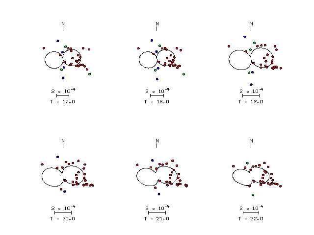
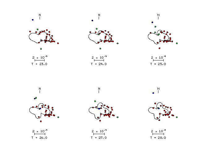
| Pressure-tension axis trends. Since the surface-wave spectra search does not distinguish between P and T axes and since there is a 180 ambiguity in strike, all possible P and T axes are plotted. First motion data and waveforms will be used to select the preferred mechanism. The purpose of this plot is to provide an idea of the possible range of solutions. The P and T-axes for all mechanisms with goodness of fit greater than 0.9 FITMAX (above) are plotted here. |

|
| Focal mechanism sensitivity at the preferred depth. The red color indicates a very good fit to the Love and Rayleigh wave radiation patterns. Each solution is plotted as a vector at a given value of strike and dip with the angle of the vector representing the rake angle, measured, with respect to the upward vertical (N) in the figure. A nearly vertical strike-slip fault striking at 75 or 165 degrees is preferred. Because of the symmetry of the spectral amplitude rediation patterns, only strikes from 0-180 degrees are sampled. |
Sta Az(deg)    Dist(km)
HAWA	  101	  155
OCWA	  301	  235
PGC	  327	  263
PNT	   25	  325
NEW	   60	  374
WSLR	  345	  397
LLLB	  356	  438
CBB	  324	  470
WVOR	  153	  525
MSO	   86	  578
HLID	  119	  657
WDC	  187	  684
BOZ	   95	  771
BBB	  324	  777
REDW	  110	  917
AHID	  114	  932
EDM	   36	  933
CMB	  174	  965
HWUT	  122	  974
DUG	  133	 1007
BW06	  110	 1041
SAO	  180	 1102
LAO	   84	 1168
DGMT	   75	 1315
DLBC	  340	 1429
ISCO	  115	 1497
WUAZ	  142	 1502
SDCO	  121	 1648
WHY	  336	 1783
YKW3	   11	 1822
ULM	   69	 1928
CBKS	  108	 1977
DAWY	  337	 2228
FCC	   44	 2265
WMOK	  117	 2321
MIAR	  110	 2700
FVM	  100	 2717
UALR	  108	 2774
LRAL	  105	 3284
ERPA	   84	 3309
BLA	   92	 3522
ACCN	   78	 3731
PAL	   82	 3822
Since the analysis of the surface-wave radiation patterns uses only spectral amplitudes and because the surfave-wave radiation patterns have a 180 degree symmetry, each surface-wave solution consists of four possible focal mechanisms corresponding to the interchange of the P- and T-axes and a roation of the mechanism by 180 degrees. To select one mechanism, P-wave first motion can be used. This was not possible in this case because all the P-wave first motions were emergent ( a feature of the P-wave wave takeoff angle, the station location and the mechanism). The other way to select among the mechanisms is to compute forward synthetics and compare the observed and predicted waveforms.
The velocity model used for the waveform fit is a modified Utah model .
The fits to the waveforms with the given mechanism are show below:

|
This figure shows the fit to the three components of motion (Z - vertical, R-radial and T - transverse). For each station and component, the observed traces is shown in red and the model predicted trace in blue. The traces represent filtered ground velocity in units of meters/sec (the peak value is printed adjacent to each trace; each pair of traces to plotted to the same scale to emphasize the difference in levels). Both synthetic and observed traces have been filtered using the SAC commands:
hp c 0.02 3
lp c 0.10 3

|

|
Should the national backbone of the USGS Advanced National Seismic System (ANSS) be implemented with an interstation separation of 300 km, it is very likely that an earthquake such as this would have been recorded at distances on the order of 100-200 km. This means that the closest station would have information on source depth and mechanism that was lacking here.
Dr. Harley Benz, USGS, provided the USGS USNSN digital data.
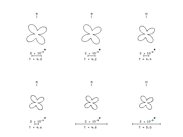
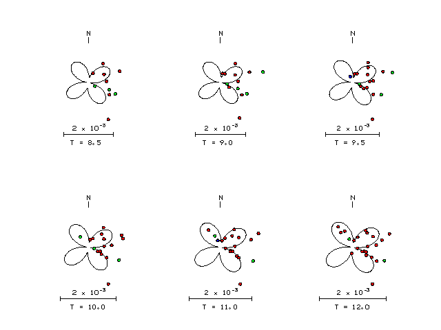
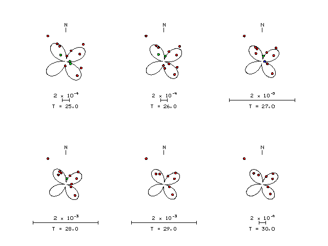
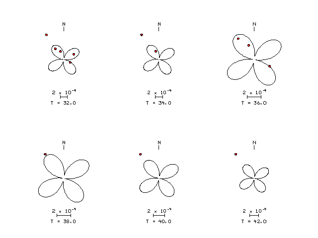
The figures below show the observed spectral amplitudes (units of cm-sec) at each station and the
theoretical predictions as a function of period for the mechanism given above. The modified Utah model earth model
was used to define the Green's functions. For each station, the Love and Rayleigh wave spectrail amplitudes are plotted with the same scaling so that one can get a sense fo the effects of the effects of the focal mechanism and depth on the excitation of each.
 |
 |
 |
 |
 |
 |
 |
 |
 |
 |
 |
 |
 |
 |
 |
 |
 |
 |
 |
 |
 |
 |
 |
 |
 |
 |
 |
 |
 |
 |
 |
 |
 |
 |
 |
 |
 |
 |
 |
 |
 |
 |
 |
Here we tabulate the reasons for not using certain digital data sets
The following stations did not have a valid response files: