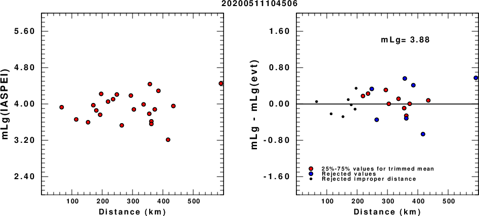
(a) mLg computed using the IASPEI formula; (b) mLg residuals ; the values used for the trimmed mean are indicated.
 USGS/SLU Moment Tensor Solution
 ENS  2020/05/11 10:45:06:0  38.68  127.18  16.0 3.8 Korea

 Stations used:
   KS.CHC2 KS.DACB KS.DAG2 KS.DGY2 KS.EMSB KS.EURB KS.GOCB
   KS.GWYB KS.HAWB KS.IMWB KS.JEO2 KS.OKCB KS.OKEB KS.SES2
   KS.SHHB KS.SMKB KS.ULJ2

 Filtering commands used:
   cut o DIST/3.3 -30 o DIST/3.3 +50
   rtr
   taper w 0.1
   hp c 0.02 n 3
   lp c 0.10 n 3

 Best Fitting Double Couple
  Mo = 3.76e+21 dyne-cm
  Mw = 3.65
  Z  = 6 km
  Plane   Strike  Dip  Rake
   NP1      135    85    20
   NP2       43    70   175
  Principal Axes:
   Axis    Value   Plunge  Azimuth
    T   3.76e+21     18       1
    N   0.00e+00     69     148
    P  -3.76e+21     10     267

 Moment Tensor: (dyne-cm)
    Component   Value
       Mxx     3.41e+21
       Mxy    -1.12e+20
       Mxz     1.11e+21
       Myy    -3.63e+21
       Myz     6.77e+20
       Mzz     2.23e+20


                     ######   #####
                 ########## T #########
              #############   ############
             -############################-
           ----###########################---
          -------########################-----
         ---------######################-------
        ------------###################---------
        --------------################----------
       ----------------##############------------
       -   --------------##########--------------
       - P ----------------#######---------------
       -   ------------------###-----------------
        ----------------------------------------
        ---------------------####---------------
         ------------------########------------
          --------------#############---------
           ----------##################------
             -----########################-
              ############################
                 ######################
                     ##############


 Global CMT Convention Moment Tensor:
      R          T          P
  2.23e+20   1.11e+21  -6.77e+20
  1.11e+21   3.41e+21   1.12e+20
 -6.77e+20   1.12e+20  -3.63e+21


Details of the solution is found at

http://www.eas.slu.edu/eqc/eqc_mt/MECH.NA/20200511104506/index.html
|
      STK = 135
      DIP = 85
     RAKE = 20
       MW = 3.65
       HS = 6.0
The NDK file is 20200511104506.ndk The waveform inversion is preferred.
The following compares this source inversion to others
 USGS/SLU Moment Tensor Solution
 ENS  2020/05/11 10:45:06:0  38.68  127.18  16.0 3.8 Korea

 Stations used:
   KS.CHC2 KS.DACB KS.DAG2 KS.DGY2 KS.EMSB KS.EURB KS.GOCB
   KS.GWYB KS.HAWB KS.IMWB KS.JEO2 KS.OKCB KS.OKEB KS.SES2
   KS.SHHB KS.SMKB KS.ULJ2

 Filtering commands used:
   cut o DIST/3.3 -30 o DIST/3.3 +50
   rtr
   taper w 0.1
   hp c 0.02 n 3
   lp c 0.10 n 3

 Best Fitting Double Couple
  Mo = 3.76e+21 dyne-cm
  Mw = 3.65
  Z  = 6 km
  Plane   Strike  Dip  Rake
   NP1      135    85    20
   NP2       43    70   175
  Principal Axes:
   Axis    Value   Plunge  Azimuth
    T   3.76e+21     18       1
    N   0.00e+00     69     148
    P  -3.76e+21     10     267

 Moment Tensor: (dyne-cm)
    Component   Value
       Mxx     3.41e+21
       Mxy    -1.12e+20
       Mxz     1.11e+21
       Myy    -3.63e+21
       Myz     6.77e+20
       Mzz     2.23e+20


                     ######   #####
                 ########## T #########
              #############   ############
             -############################-
           ----###########################---
          -------########################-----
         ---------######################-------
        ------------###################---------
        --------------################----------
       ----------------##############------------
       -   --------------##########--------------
       - P ----------------#######---------------
       -   ------------------###-----------------
        ----------------------------------------
        ---------------------####---------------
         ------------------########------------
          --------------#############---------
           ----------##################------
             -----########################-
              ############################
                 ######################
                     ##############


 Global CMT Convention Moment Tensor:
      R          T          P
  2.23e+20   1.11e+21  -6.77e+20
  1.11e+21   3.41e+21   1.12e+20
 -6.77e+20   1.12e+20  -3.63e+21


Details of the solution is found at

http://www.eas.slu.edu/eqc/eqc_mt/MECH.NA/20200511104506/index.html
|
(a) mLg computed using the IASPEI formula; (b) mLg residuals ; the values used for the trimmed mean are indicated.
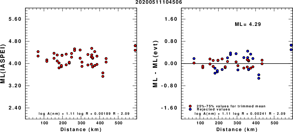
(a) ML computed using the IASPEI formula for Horizontal components; (b) ML residuals computed using a modified IASPEI formula that accounts for path specific attenuation; the values used for the trimmed mean are indicated. The ML relation used for each figure is given at the bottom of each plot.
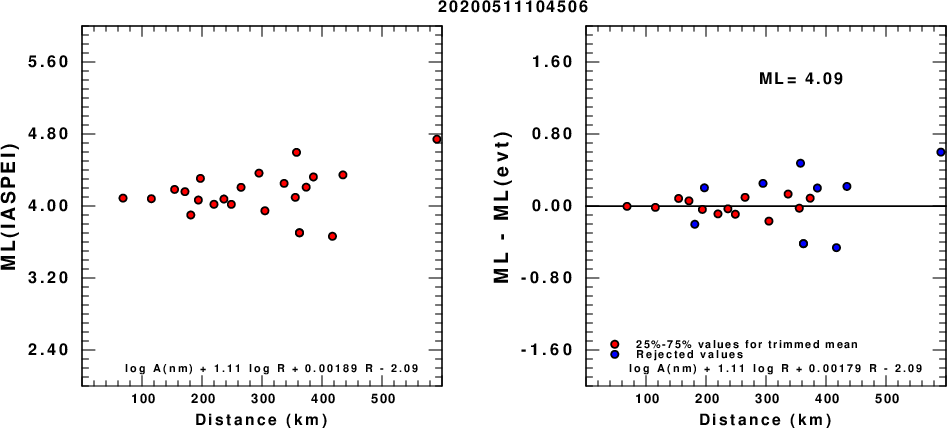
(a) ML computed using the IASPEI formula for Vertical components (research); (b) ML residuals computed using a modified IASPEI formula that accounts for path specific attenuation; the values used for the trimmed mean are indicated. The ML relation used for each figure is given at the bottom of each plot.
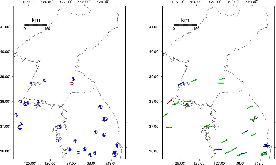 |
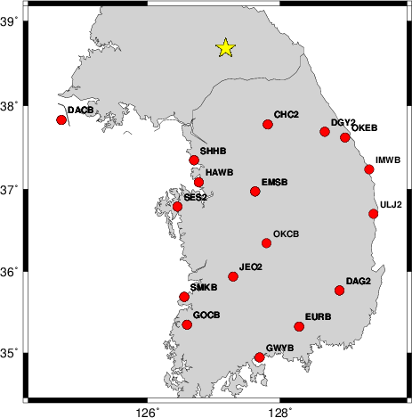
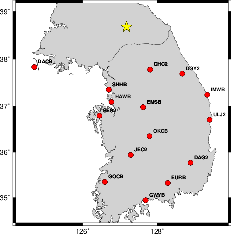
The focal mechanism was determined using broadband seismic waveforms. The location of the event and the and stations used for the waveform inversion are shown in the next figure.
|
|
|
The program wvfgrd96 was used with good traces observed at short distance to determine the focal mechanism, depth and seismic moment. This technique requires a high quality signal and well determined velocity model for the Green functions. To the extent that these are the quality data, this type of mechanism should be preferred over the radiation pattern technique which requires the separate step of defining the pressure and tension quadrants and the correct strike.
The observed and predicted traces are filtered using the following gsac commands:
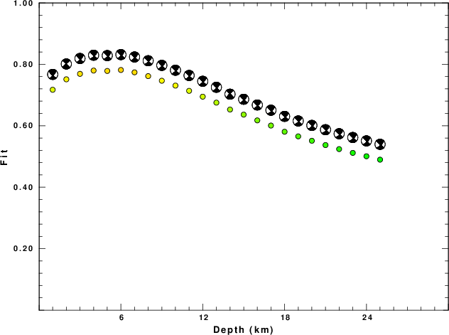
cut o DIST/3.3 -30 o DIST/3.3 +50
rtr
taper w 0.1
hp c 0.02 n 3
lp c 0.10 n 3
The results of this grid search from 0.5 to 19 km depth are as follow:
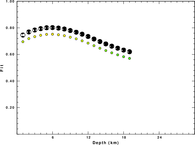
           DEPTH  STK   DIP  RAKE   MW    FIT
WVFGRD96    1.0   135    75    20   3.57 0.7172
WVFGRD96    2.0   135    90    -5   3.58 0.7512
WVFGRD96    3.0   135    80    20   3.61 0.7690
WVFGRD96    4.0   135    85    20   3.63 0.7797
WVFGRD96    5.0   315    90   -20   3.64 0.7784
WVFGRD96    6.0   135    85    20   3.65 0.7816
WVFGRD96    7.0   135    85    15   3.66 0.7739
WVFGRD96    8.0   135    85    15   3.67 0.7616
WVFGRD96    9.0   135    85    15   3.68 0.7466
WVFGRD96   10.0   135    85    15   3.68 0.7308
WVFGRD96   11.0   135    85    15   3.69 0.7137
WVFGRD96   12.0   135    85    15   3.70 0.6948
WVFGRD96   13.0   135    85    15   3.71 0.6753
WVFGRD96   14.0   315    85    10   3.72 0.6528
WVFGRD96   15.0   135    85    15   3.73 0.6363
WVFGRD96   16.0   135    85    15   3.74 0.6176
WVFGRD96   17.0   135    85    20   3.75 0.6007
WVFGRD96   18.0   315    90   -20   3.76 0.5806
WVFGRD96   19.0   315    90   -15   3.76 0.5656
WVFGRD96   20.0   315    90   -15   3.78 0.5512
WVFGRD96   21.0   315    90   -20   3.79 0.5372
WVFGRD96   22.0   135    85    20   3.80 0.5241
WVFGRD96   23.0   135    90    20   3.81 0.5118
WVFGRD96   24.0   135    90    20   3.82 0.5008
WVFGRD96   25.0   135    90    20   3.83 0.4897
The best solution is
WVFGRD96 6.0 135 85 20 3.65 0.7816
The mechanism correspond to the best fit is
|
|
|
The best fit as a function of depth is given in the following figure:
|
|
|
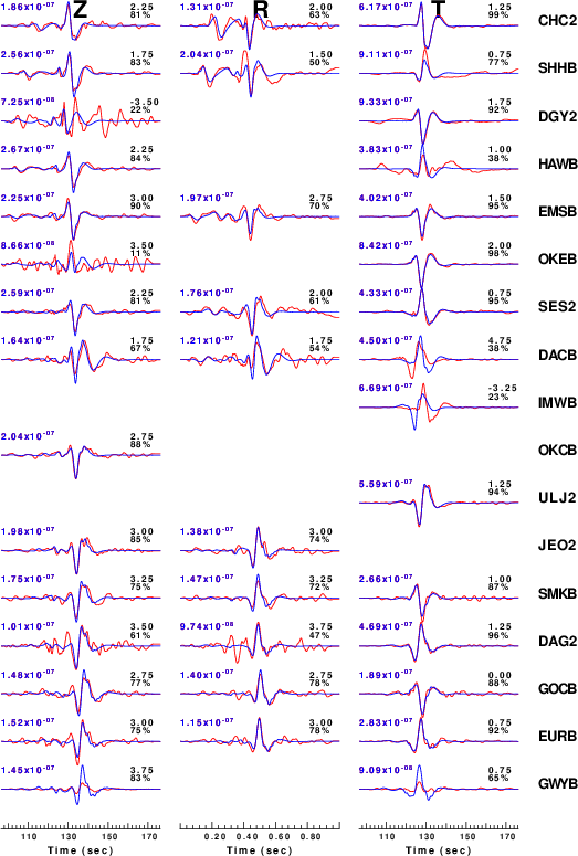
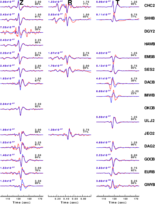
The comparison of the observed and predicted waveforms is given in the next figure. The red traces are the observed and the blue are the predicted. Each observed-predicted component is plotted to the same scale and peak amplitudes are indicated by the numbers to the left of each trace. A pair of numbers is given in black at the right of each predicted traces. The upper number it the time shift required for maximum correlation between the observed and predicted traces. This time shift is required because the synthetics are not computed at exactly the same distance as the observed and because the velocity model used in the predictions may not be perfect. A positive time shift indicates that the prediction is too fast and should be delayed to match the observed trace (shift to the right in this figure). A negative value indicates that the prediction is too slow. The lower number gives the percentage of variance reduction to characterize the individual goodness of fit (100% indicates a perfect fit).
The bandpass filter used in the processing and for the display was
cut o DIST/3.3 -30 o DIST/3.3 +50
rtr
taper w 0.1
hp c 0.02 n 3
lp c 0.10 n 3
|
|
|
|
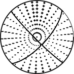
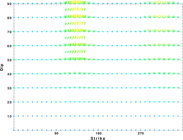
| Focal mechanism sensitivity at the preferred depth. The red color indicates a very good fit to thewavefroms. Each solution is plotted as a vector at a given value of strike and dip with the angle of the vector representing the rake angle, measured, with respect to the upward vertical (N) in the figure. |
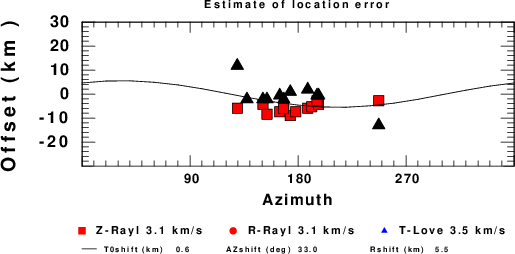
A check on the assumed source location is possible by looking at the time shifts between the observed and predicted traces. The time shifts for waveform matching arise for several reasons:
Time_shift = A + B cos Azimuth + C Sin Azimuth
The time shifts for this inversion lead to the next figure:
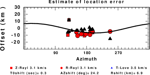
The derived shift in origin time and epicentral coordinates are given at the bottom of the figure.
The focal mechanism was determined using broadband seismic waveforms. The location of the event and the and stations used for the waveform inversion are shown in the next figure.
|
|
|
The program wvfmtgrd96 was used with good traces observed at short distance to determine the focal mechanism, depth and seismic moment. This technique requires a high quality signal and well determined velocity model for the Green functions. To the extent that these are the quality data, this type of mechanism should be preferred over the radiation pattern technique which requires the separate step of defining the pressure and tension quadrants and the correct strike.
The observed and predicted traces are filtered using the following gsac commands:
cut o DIST/3.3 -30 o DIST/3.3 +50
rtr
taper w 0.1
hp c 0.02 n 3
lp c 0.10 n 3
The results of this grid search over depth are as follow:
MT Program  H(km) Mxx(dyne-cm)   Myy        Mxy        Mxz        Myz        Mzz       Mw      Fit
WVFMTGRD96    1.0  0.162E+22 -0.388E+22 -0.290E+21 -0.426E+20 -0.114E+22 -0.138E+22  3.6162  0.6958
WVFMTGRD96    2.0  0.260E+22 -0.340E+22 -0.358E+21  0.427E+21 -0.299E+21  0.135E+22  3.6065  0.7192
WVFMTGRD96    3.0  0.274E+22 -0.363E+22 -0.393E+21  0.985E+21  0.474E+21  0.597E+21  3.6251  0.7337
WVFMTGRD96    4.0  0.318E+22 -0.350E+22 -0.412E+21  0.103E+22  0.497E+21  0.933E+21  3.6393  0.7440
WVFMTGRD96    5.0  0.362E+22 -0.331E+22 -0.428E+21  0.107E+22  0.515E+21  0.129E+22  3.6536  0.7507
WVFMTGRD96    6.0  0.427E+22 -0.294E+22 -0.457E+21  0.102E+22  0.571E+21  0.205E+22  3.6778  0.7520
WVFMTGRD96    7.0  0.472E+22 -0.279E+22 -0.482E+21  0.101E+22  0.612E+21  0.252E+22  3.6991  0.7482
WVFMTGRD96    8.0  0.507E+22 -0.268E+22 -0.498E+21  0.105E+22  0.633E+21  0.280E+22  3.7150  0.7411
WVFMTGRD96    9.0  0.553E+22 -0.244E+22 -0.512E+21  0.108E+22  0.651E+21  0.320E+22  3.7341  0.7297
WVFMTGRD96   10.0  0.571E+22 -0.262E+22 -0.550E+21  0.102E+22  0.721E+21  0.352E+22  3.7479  0.7173
WVFMTGRD96   11.0  0.615E+22 -0.242E+22 -0.565E+21  0.105E+22  0.741E+21  0.389E+22  3.7655  0.7024
WVFMTGRD96   12.0  0.669E+22 -0.215E+22 -0.583E+21  0.108E+22  0.765E+21  0.436E+22  3.7866  0.6851
WVFMTGRD96   13.0  0.722E+22 -0.183E+22 -0.597E+21  0.110E+22  0.783E+21  0.484E+22  3.8063  0.6660
WVFMTGRD96   14.0  0.706E+22 -0.227E+22 -0.615E+21  0.114E+22  0.807E+21  0.460E+22  3.8020  0.6467
WVFMTGRD96   15.0  0.762E+22 -0.193E+22 -0.630E+21  0.117E+22  0.827E+21  0.511E+22  3.8221  0.6292
WVFMTGRD96   16.0  0.611E+22 -0.376E+22 -0.470E+21  0.115E+22  0.106E+22  0.450E+22  3.7952  0.6122
WVFMTGRD96   17.0  0.705E+22 -0.301E+22 -0.455E+21  0.135E+22  0.104E+22  0.517E+22  3.8205  0.5970
WVFMTGRD96   18.0  0.665E+22 -0.362E+22 -0.478E+21  0.146E+22  0.167E+22  0.492E+22  3.8206  0.5829
WVFMTGRD96   19.0  0.686E+22 -0.374E+22 -0.493E+21  0.151E+22  0.172E+22  0.507E+22  3.8296  0.5704
The best solution is
WVFMTGRD96 6.0 0.427E+22 -0.294E+22 -0.457E+21 0.102E+22 0.571E+21 0.205E+22 3.6778 0.7520
The complete moment tensor decomposition using the program mtinfo is given in the text file MTGRDinfo.txt. (Jost, M. L., and R. B. Herrmann (1989). A student's guide to and review of moment tensors, Seism. Res. Letters 60, 37-57. SRL_60_2_37-57.pdf.
The P-wave first motion mechanism corresponding to the best fit is
|
|
|
The best fit as a function of depth is given in the following figure:
|
|
|
The comparison of the observed and predicted waveforms is given in the next figure. The red traces are the observed and the blue are the predicted. Each observed-predicted component is plotted to the same scale and peak amplitudes are indicated by the numbers to the left of each trace. A pair of numbers is given in black at the right of each predicted traces. The upper number it the time shift required for maximum correlation between the observed and predicted traces. This time shift is required because the synthetics are not computed at exactly the same distance as the observed and because the velocity model used in the predictions may not be perfect. A positive time shift indicates that the prediction is too fast and should be delayed to match the observed trace (shift to the right in this figure). A negative value indicates that the prediction is too slow. The lower number gives the percentage of variance reduction to characterize the individual goodness of fit (100% indicates a perfect fit).
The bandpass filter used in the processing and for the display was
cut o DIST/3.3 -30 o DIST/3.3 +50
rtr
taper w 0.1
hp c 0.02 n 3
lp c 0.10 n 3
|
|
|
A check on the assumed source location is possible by looking at the time shifts between the observed and predicted traces. The time shifts for waveform matching arise for several reasons:
Time_shift = A + B cos Azimuth + C Sin Azimuth
The time shifts for this inversion lead to the next figure:
The derived shift in origin time and epicentral coordinates are given at the bottom of the figure.
Thanks also to the many seismic network operators whose dedication make this effort possible: University of Nevada Reno, University of Alaska, University of Washington, Oregon State University, University of Utah, Montana Bureau of Mines, UC Berkely, Caltech, UC San Diego, Saint Louis University, University of Memphis, Lamont Doherty Earth Observatory, the Oklahoma Geological Survey, TexNet, the Iris stations, the Transportable Array of EarthScope and other networks.
The t6.invSNU.CUVEL model used for the waveform synthetic seismograms and for the surface wave eigenfunctions and dispersion is as follows:
MODEL.01
Model after    30 iterations
ISOTROPIC
KGS
SPHERICAL EARTH
1-D
CONSTANT VELOCITY
LINE08
LINE09
LINE10
LINE11
      H(KM)   VP(KM/S)   VS(KM/S) RHO(GM/CC)         QP         QS       ETAP       ETAS      FREFP      FREFS
     1.0000     5.3800     3.0009     2.5772  0.118E-02  0.167E-02   0.00       0.00       1.00       1.00
     1.0000     5.8057     3.2383     2.6606  0.118E-02  0.167E-02   0.00       0.00       1.00       1.00
     1.0000     6.1732     3.4433     2.7513  0.118E-02  0.167E-02   0.00       0.00       1.00       1.00
     3.0000     6.2872     3.5067     2.7862  0.118E-02  0.167E-02   0.00       0.00       1.00       1.00
     5.0000     6.3245     3.5281     2.7970  0.118E-02  0.167E-02   0.00       0.00       1.00       1.00
     5.0000     6.4165     3.5788     2.8248  0.118E-02  0.167E-02   0.00       0.00       1.00       1.00
     4.0000     6.5576     3.6576     2.8653  0.118E-02  0.167E-02   0.00       0.00       1.00       1.00
     5.0000     6.6402     3.7038     2.8865  0.118E-02  0.167E-02   0.00       0.00       1.00       1.00
     2.5000     6.6540     3.7115     2.8897  0.118E-02  0.167E-02   0.00       0.00       1.00       1.00
     2.5000     7.0960     3.9579     3.0111  0.118E-02  0.167E-02   0.00       0.00       1.00       1.00
     2.5000     7.9155     4.4148     3.2804  0.118E-02  0.167E-02   0.00       0.00       1.00       1.00
     2.5000     7.8925     4.4019     3.2735  0.118E-02  0.167E-02   0.00       0.00       1.00       1.00
     5.0000     7.8665     4.3876     3.2643  0.118E-02  0.167E-02   0.00       0.00       1.00       1.00
     5.0000     7.5675     4.2211     3.1625  0.118E-02  0.167E-02   0.00       0.00       1.00       1.00
     5.0000     7.7550     4.3252     3.2262  0.118E-02  0.167E-02   0.00       0.00       1.00       1.00
     5.0000     7.7602     4.3280     3.2282  0.118E-02  0.167E-02   0.00       0.00       1.00       1.00
     5.0000     7.7958     4.3487     3.2398  0.118E-02  0.167E-02   0.00       0.00       1.00       1.00
     5.0000     7.7415     4.3195     3.2217  0.118E-02  0.167E-02   0.00       0.00       1.00       1.00
     5.0000     7.6497     4.2688     3.1915  0.118E-02  0.167E-02   0.00       0.00       1.00       1.00
     5.0000     7.6408     4.2653     3.1889  0.118E-02  0.167E-02   0.00       0.00       1.00       1.00
     5.0000     7.6666     4.2716     3.1976  0.118E-02  0.167E-02   0.00       0.00       1.00       1.00
     5.0000     7.6699     4.2830     3.1986  0.118E-02  0.167E-02   0.00       0.00       1.00       1.00
     5.0000     7.6780     4.2885     3.2014  0.118E-02  0.167E-02   0.00       0.00       1.00       1.00
     5.0000     7.6816     4.2896     3.2028  0.118E-02  0.167E-02   0.00       0.00       1.00       1.00
     5.0000     7.6946     4.2996     3.2072  0.118E-02  0.167E-02   0.00       0.00       1.00       1.00
    10.0000     7.7349     4.3197     3.2208  0.118E-02  0.167E-02   0.00       0.00       1.00       1.00
    10.0000     7.7791     4.3484     3.2355  0.118E-02  0.167E-02   0.00       0.00       1.00       1.00
    10.0000     7.8331     4.3722     3.2536  0.862E-02  0.131E-01   0.00       0.00       1.00       1.00
    10.0000     7.8824     4.3863     3.2703  0.862E-02  0.131E-01   0.00       0.00       1.00       1.00
    10.0000     7.9360     4.4024     3.2883  0.855E-02  0.131E-01   0.00       0.00       1.00       1.00
    10.0000     7.9967     4.4237     3.3088  0.847E-02  0.131E-01   0.00       0.00       1.00       1.00
    10.0000     8.0529     4.4423     3.3289  0.847E-02  0.131E-01   0.00       0.00       1.00       1.00
    10.0000     8.1110     4.4603     3.3496  0.833E-02  0.130E-01   0.00       0.00       1.00       1.00
    10.0000     8.1762     4.4832     3.3728  0.826E-02  0.129E-01   0.00       0.00       1.00       1.00
    10.0000     8.2410     4.5054     3.3959  0.813E-02  0.128E-01   0.00       0.00       1.00       1.00
    10.0000     8.3022     4.5257     3.4176  0.806E-02  0.126E-01   0.00       0.00       1.00       1.00
    10.0000     8.3635     4.5514     3.4395  0.474E-02  0.746E-02   0.00       0.00       1.00       1.00
    10.0000     8.4257     4.5839     3.4617  0.472E-02  0.741E-02   0.00       0.00       1.00       1.00
    10.0000     8.4845     4.6145     3.4827  0.469E-02  0.741E-02   0.00       0.00       1.00       1.00
    10.0000     8.5403     4.6434     3.5020  0.467E-02  0.735E-02   0.00       0.00       1.00       1.00
    10.0000     8.5934     4.6708     3.5199  0.465E-02  0.735E-02   0.00       0.00       1.00       1.00
    10.0000     8.6436     4.6959     3.5369  0.463E-02  0.730E-02   0.00       0.00       1.00       1.00
    10.0000     8.6912     4.7194     3.5530  0.461E-02  0.730E-02   0.00       0.00       1.00       1.00
    10.0000     8.7365     4.7413     3.5684  0.459E-02  0.725E-02   0.00       0.00       1.00       1.00
    10.0000     8.7797     4.7622     3.5831  0.455E-02  0.725E-02   0.00       0.00       1.00       1.00
    10.0000     8.8199     4.7819     3.5967  0.452E-02  0.719E-02   0.00       0.00       1.00       1.00
    10.0000     8.8587     4.8001     3.6099  0.450E-02  0.714E-02   0.00       0.00       1.00       1.00
    10.0000     8.8958     4.8177     3.6226  0.448E-02  0.714E-02   0.00       0.00       1.00       1.00
    10.0000     8.9314     4.8346     3.6347  0.446E-02  0.709E-02   0.00       0.00       1.00       1.00
    10.0000     8.9647     4.8500     3.6461  0.442E-02  0.704E-02   0.00       0.00       1.00       1.00
    10.0000     8.9962     4.8651     3.6569  0.441E-02  0.704E-02   0.00       0.00       1.00       1.00
    10.0000     9.0263     4.8783     3.6685  0.439E-02  0.699E-02   0.00       0.00       1.00       1.00
    10.0000     9.0547     4.8915     3.6800  0.435E-02  0.694E-02   0.00       0.00       1.00       1.00
    10.0000     9.0822     4.9041     3.6911  0.433E-02  0.690E-02   0.00       0.00       1.00       1.00
    10.0000     9.1091     4.9164     3.7020  0.431E-02  0.690E-02   0.00       0.00       1.00       1.00
    10.0000     9.1346     4.9280     3.7123  0.427E-02  0.685E-02   0.00       0.00       1.00       1.00
    10.0000     9.4876     5.1513     3.8537  0.388E-02  0.613E-02   0.00       0.00       1.00       1.00
    10.0000     9.5095     5.1663     3.8624  0.388E-02  0.613E-02   0.00       0.00       1.00       1.00
    10.0000     9.5299     5.1806     3.8703  0.386E-02  0.610E-02   0.00       0.00       1.00       1.00
    10.0000     9.5507     5.1944     3.8784  0.386E-02  0.610E-02   0.00       0.00       1.00       1.00
    10.0000     9.5706     5.2080     3.8861  0.385E-02  0.606E-02   0.00       0.00       1.00       1.00
    10.0000     9.5900     5.2214     3.8937  0.385E-02  0.606E-02   0.00       0.00       1.00       1.00
    10.0000     9.6090     5.2347     3.9011  0.383E-02  0.606E-02   0.00       0.00       1.00       1.00
    10.0000     9.6272     5.2480     3.9081  0.383E-02  0.602E-02   0.00       0.00       1.00       1.00
    10.0000     9.6458     5.2604     3.9154  0.383E-02  0.602E-02   0.00       0.00       1.00       1.00
    10.0000     9.6794     5.2816     3.9282  0.382E-02  0.599E-02   0.00       0.00       1.00       1.00
    10.0000     9.7130     5.3029     3.9409  0.382E-02  0.599E-02   0.00       0.00       1.00       1.00
    10.0000     9.7466     5.3242     3.9537  0.380E-02  0.599E-02   0.00       0.00       1.00       1.00
    10.0000     9.7799     5.3454     3.9664  0.380E-02  0.595E-02   0.00       0.00       1.00       1.00
    10.0000     9.8137     5.3669     3.9792  0.380E-02  0.595E-02   0.00       0.00       1.00       1.00
    10.0000     9.8473     5.3883     3.9920  0.379E-02  0.592E-02   0.00       0.00       1.00       1.00
    10.0000     9.8808     5.4094     4.0047  0.379E-02  0.592E-02   0.00       0.00       1.00       1.00
     0.0000     9.9144     5.4306     4.0175  0.377E-02  0.592E-02   0.00       0.00       1.00       1.00
Here we tabulate the reasons for not using certain digital data sets
The following stations did not have a valid response files: