Location

SLU location

First arrival times and P-wave first motions were picked, and the earthquake was located using the velocity model given below. The purpose was to check the conssitency between the waveform inversion focal mechanism and the observed P-wave first motions. The program elocate was used. The file elocate.txt give the observations and the result of running the location program.

KMA Location

2018/02/10 20:03:03 36.08 129.33 14.0 4.6 Korea

Focal Mechanism

USGS/SLU Moment Tensor Solution ENS 2018/02/10 20:03:03:0 36.08 129.33 14.0 4.6 Korea Stations used: IU.INCN KG.TJN KS.BOSB KS.BUS2 KS.CHC2 KS.CHJ2 KS.DACB KS.DAG2 KS.DGY2 KS.EMSB KS.EURB KS.GAHB KS.GOCB KS.GWYB KS.HALB KS.HAMB KS.HAWB KS.HWCB KS.IMWB KS.JEO2 KS.KOHB KS.NAWB KS.OKCB KS.OKEB KS.SEHB KS.SEO2 KS.SES2 KS.SHHB KS.SMKB KS.ULJ2 KS.YNCB Filtering commands used: cut o DIST/3.3 -30 o DIST/3.3 +40 rtr taper w 0.1 hp c 0.02 n 3 lp c 0.10 n 3 Best Fitting Double Couple Mo = 1.07e+23 dyne-cm Mw = 4.62 Z = 5 km Plane Strike Dip Rake NP1 20 55 120 NP2 155 45 55 Principal Axes: Axis Value Plunge Azimuth T 1.07e+23 65 348 N 0.00e+00 24 181 P -1.07e+23 5 89 Moment Tensor: (dyne-cm) Component Value Mxx 1.76e+22 Mxy -5.68e+21 Mxz 3.94e+22 Myy -1.05e+23 Myz -1.84e+22 Mzz 8.78e+22 ############## -##################--- ---####################----- ---######################----- -----######################------- ------######################-------- ------########## ##########--------- -------########## T ##########---------- -------########## ##########---------- ---------######################-------- ---------######################-------- P ---------#####################--------- ----------###################------------- ----------##################------------ -----------################------------- -----------##############------------- -----------############------------- ------------########-------------- ------------#####------------- -------------#-------------- --------######-------- ############## Global CMT Convention Moment Tensor: R T P 8.78e+22 3.94e+22 1.84e+22 3.94e+22 1.76e+22 5.68e+21 1.84e+22 5.68e+21 -1.05e+23 Details of the solution is found at http://www.eas.slu.edu/eqc/eqc_mt/MECH.NA/20180210200303/index.html

Preferred Solution

The preferred solution from an analysis of the surface-wave spectral amplitude radiation pattern, waveform inversion and first motion observations is

      STK = 155
      DIP = 45
     RAKE = 55
       MW = 4.62
       HS = 5.0

The NDK file is 20180210200303.ndk The waveform inversion is preferred.

Moment Tensor Comparison

The following compares this source inversion to others

SLU SLUFM

USGS/SLU Moment Tensor Solution ENS 2018/02/10 20:03:03:0 36.08 129.33 14.0 4.6 Korea Stations used: IU.INCN KG.TJN KS.BOSB KS.BUS2 KS.CHC2 KS.CHJ2 KS.DACB KS.DAG2 KS.DGY2 KS.EMSB KS.EURB KS.GAHB KS.GOCB KS.GWYB KS.HALB KS.HAMB KS.HAWB KS.HWCB KS.IMWB KS.JEO2 KS.KOHB KS.NAWB KS.OKCB KS.OKEB KS.SEHB KS.SEO2 KS.SES2 KS.SHHB KS.SMKB KS.ULJ2 KS.YNCB Filtering commands used: cut o DIST/3.3 -30 o DIST/3.3 +40 rtr taper w 0.1 hp c 0.02 n 3 lp c 0.10 n 3 Best Fitting Double Couple Mo = 1.07e+23 dyne-cm Mw = 4.62 Z = 5 km Plane Strike Dip Rake NP1 20 55 120 NP2 155 45 55 Principal Axes: Axis Value Plunge Azimuth T 1.07e+23 65 348 N 0.00e+00 24 181 P -1.07e+23 5 89 Moment Tensor: (dyne-cm) Component Value Mxx 1.76e+22 Mxy -5.68e+21 Mxz 3.94e+22 Myy -1.05e+23 Myz -1.84e+22 Mzz 8.78e+22 ############## -##################--- ---####################----- ---######################----- -----######################------- ------######################-------- ------########## ##########--------- -------########## T ##########---------- -------########## ##########---------- ---------######################-------- ---------######################-------- P ---------#####################--------- ----------###################------------- ----------##################------------ -----------################------------- -----------##############------------- -----------############------------- ------------########-------------- ------------#####------------- -------------#-------------- --------######-------- ############## Global CMT Convention Moment Tensor: R T P 8.78e+22 3.94e+22 1.84e+22 3.94e+22 1.76e+22 5.68e+21 1.84e+22 5.68e+21 -1.05e+23 Details of the solution is found at http://www.eas.slu.edu/eqc/eqc_mt/MECH.NA/20180210200303/index.html

First motions and takeoff angles from an elocate run.

Magnitudes

mLg Magnitude

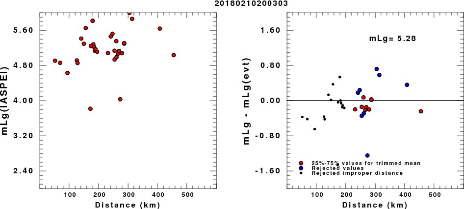
(a) mLg computed using the IASPEI formula; (b) mLg residuals ; the values used for the trimmed mean are indicated.

ML Magnitude

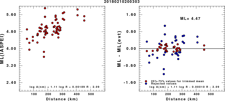
(a) ML computed using the IASPEI formula; (b) ML residuals computed using a modified IASPEI formula that accounts for path specific attenuation; the values used for the trimmed mean are indicated. The ML relation used for each figure is given at the bottom of each plot.

Waveform Inversion

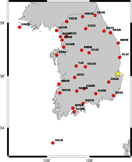
The focal mechanism was determined using broadband seismic waveforms. The location of the event and the and stations used for the waveform inversion are shown in the next figure.

Location of broadband stations used for waveform inversion

The program wvfgrd96 was used with good traces observed at short distance to determine the focal mechanism, depth and seismic moment. This technique requires a high quality signal and well determined velocity model for the Green functions. To the extent that these are the quality data, this type of mechanism should be preferred over the radiation pattern technique which requires the separate step of defining the pressure and tension quadrants and the correct strike.

The observed and predicted traces are filtered using the following gsac commands:

cut o DIST/3.3 -30 o DIST/3.3 +40
rtr
taper w 0.1
hp c 0.02 n 3 
lp c 0.10 n 3

The results of this grid search from 0.5 to 19 km depth are as follow:

           DEPTH  STK   DIP  RAKE   MW    FIT
WVFGRD96    1.0   135    40     5   4.53 0.4536
WVFGRD96    2.0   135    40    10   4.54 0.4800
WVFGRD96    3.0   145    45    30   4.57 0.5206
WVFGRD96    4.0   155    45    50   4.62 0.5694
WVFGRD96    5.0   155    45    55   4.62 0.5769
WVFGRD96    6.0   145    50    35   4.58 0.5495
WVFGRD96    7.0   140    55    25   4.57 0.5260
WVFGRD96    8.0   140    55    20   4.56 0.5007
WVFGRD96    9.0   135    60    10   4.56 0.4784
WVFGRD96   10.0   135    65    10   4.57 0.4571
WVFGRD96   11.0   135    65    10   4.57 0.4373
WVFGRD96   12.0   135    65    10   4.58 0.4178
WVFGRD96   13.0   135    65    10   4.58 0.4012
WVFGRD96   14.0   310    70   -15   4.58 0.3861
WVFGRD96   15.0   310    70   -15   4.59 0.3745
WVFGRD96   16.0   310    70   -15   4.60 0.3623
WVFGRD96   17.0   310    70   -15   4.61 0.3500
WVFGRD96   18.0   310    70   -15   4.61 0.3381
WVFGRD96   19.0   310    70   -15   4.62 0.3274
WVFGRD96   20.0   310    70   -15   4.63 0.3170
WVFGRD96   21.0   315    75   -15   4.64 0.3073
WVFGRD96   22.0   315    75   -15   4.65 0.2985
WVFGRD96   23.0   315    75   -15   4.66 0.2907
WVFGRD96   24.0   315    75   -15   4.67 0.2838
WVFGRD96   25.0   315    75   -15   4.68 0.2769

The best solution is

WVFGRD96    5.0   155    45    55   4.62 0.5769

The mechanism correspond to the best fit is

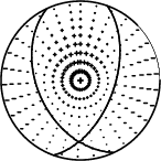
Figure 1. Waveform inversion focal mechanism

The best fit as a function of depth is given in the following figure:

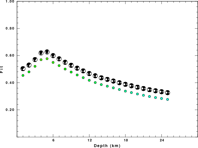
Figure 2. Depth sensitivity for waveform mechanism

The comparison of the observed and predicted waveforms is given in the next figure. The red traces are the observed and the blue are the predicted. Each observed-predicted component is plotted to the same scale and peak amplitudes are indicated by the numbers to the left of each trace. A pair of numbers is given in black at the right of each predicted traces. The upper number it the time shift required for maximum correlation between the observed and predicted traces. This time shift is required because the synthetics are not computed at exactly the same distance as the observed and because the velocity model used in the predictions may not be perfect. A positive time shift indicates that the prediction is too fast and should be delayed to match the observed trace (shift to the right in this figure). A negative value indicates that the prediction is too slow. The lower number gives the percentage of variance reduction to characterize the individual goodness of fit (100% indicates a perfect fit).

The bandpass filter used in the processing and for the display was

cut o DIST/3.3 -30 o DIST/3.3 +40
rtr
taper w 0.1
hp c 0.02 n 3 
lp c 0.10 n 3

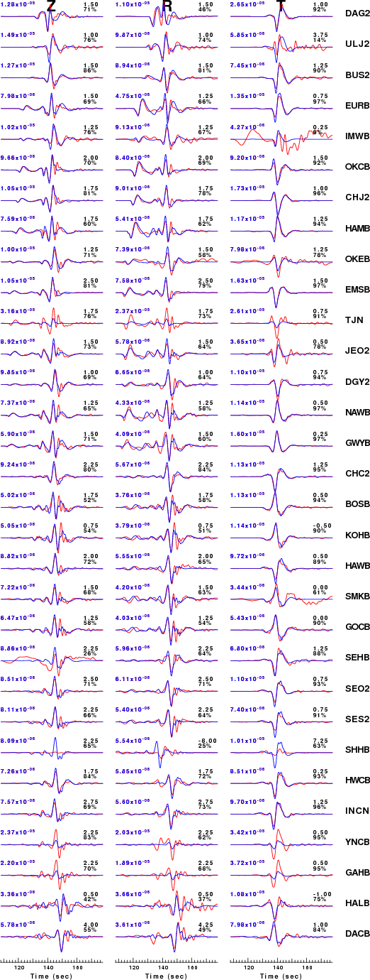
Figure 3. Waveform comparison for selected depth. Red: observed; Blue - predicted. The time shift with respect to the model prediction is indicated. The percent of fit is also indicated.

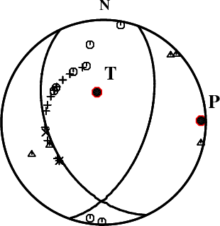
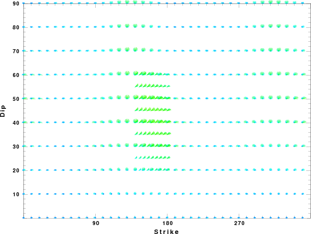
Focal mechanism sensitivity at the preferred depth. The red color indicates a very good fit to thewavefroms. Each solution is plotted as a vector at a given value of strike and dip with the angle of the vector representing the rake angle, measured, with respect to the upward vertical (N) in the figure.

A check on the assumed source location is possible by looking at the time shifts between the observed and predicted traces. The time shifts for waveform matching arise for several reasons:

The origin time and epicentral distance are incorrect
The velocity model used for the inversion is incorrect
The velocity model used to define the P-arrival time is not the same as the velocity model used for the waveform inversion (assuming that the initial trace alignment is based on the P arrival time)

Assuming only a mislocation, the time shifts are fit to a functional form:

 Time_shift = A + B cos Azimuth + C Sin Azimuth

The time shifts for this inversion lead to the next figure:

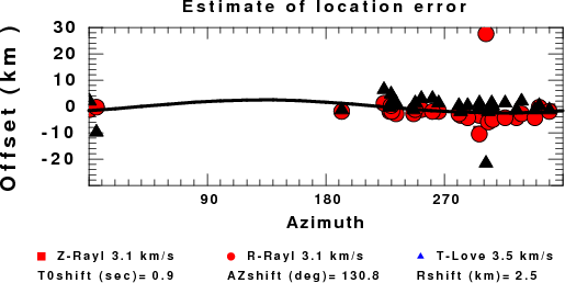
The derived shift in origin time and epicentral coordinates are given at the bottom of the figure.

Discussion

Acknowledgements

Thanks also to the many seismic network operators whose dedication make this effort possible: University of Nevada Reno, University of Alaska, University of Washington, Oregon State University, University of Utah, Montana Bureas of Mines, UC Berkely, Caltech, UC San Diego, Saint Louis University, University of Memphis, Lamont Doherty Earth Observatory, the Iris stations and the Transportable Array of EarthScope.

Velocity Model

The t6.invSNU.CUVEL.model was used for the waveform synthetic seismograms and for the surface wave eigenfunctions and dispersion is as follows:

MODEL.01
Model after    30 iterations
ISOTROPIC
KGS
SPHERICAL EARTH
1-D
CONSTANT VELOCITY
LINE08
LINE09
LINE10
LINE11
      H(KM)   VP(KM/S)   VS(KM/S) RHO(GM/CC)         QP         QS       ETAP       ETAS      FREFP      FREFS
     1.0000     5.3800     3.0009     2.5772  0.118E-02  0.167E-02   0.00       0.00       1.00       1.00    
     1.0000     5.8057     3.2383     2.6606  0.118E-02  0.167E-02   0.00       0.00       1.00       1.00    
     1.0000     6.1732     3.4433     2.7513  0.118E-02  0.167E-02   0.00       0.00       1.00       1.00    
     3.0000     6.2872     3.5067     2.7862  0.118E-02  0.167E-02   0.00       0.00       1.00       1.00    
     5.0000     6.3245     3.5281     2.7970  0.118E-02  0.167E-02   0.00       0.00       1.00       1.00    
     5.0000     6.4165     3.5788     2.8248  0.118E-02  0.167E-02   0.00       0.00       1.00       1.00    
     4.0000     6.5576     3.6576     2.8653  0.118E-02  0.167E-02   0.00       0.00       1.00       1.00    
     5.0000     6.6402     3.7038     2.8865  0.118E-02  0.167E-02   0.00       0.00       1.00       1.00    
     2.5000     6.6540     3.7115     2.8897  0.118E-02  0.167E-02   0.00       0.00       1.00       1.00    
     2.5000     7.0960     3.9579     3.0111  0.118E-02  0.167E-02   0.00       0.00       1.00       1.00    
     2.5000     7.9155     4.4148     3.2804  0.118E-02  0.167E-02   0.00       0.00       1.00       1.00    
     2.5000     7.8925     4.4019     3.2735  0.118E-02  0.167E-02   0.00       0.00       1.00       1.00    
     5.0000     7.8665     4.3876     3.2643  0.118E-02  0.167E-02   0.00       0.00       1.00       1.00    
     5.0000     7.5675     4.2211     3.1625  0.118E-02  0.167E-02   0.00       0.00       1.00       1.00    
     5.0000     7.7550     4.3252     3.2262  0.118E-02  0.167E-02   0.00       0.00       1.00       1.00    
     5.0000     7.7602     4.3280     3.2282  0.118E-02  0.167E-02   0.00       0.00       1.00       1.00    
     5.0000     7.7958     4.3487     3.2398  0.118E-02  0.167E-02   0.00       0.00       1.00       1.00    
     5.0000     7.7415     4.3195     3.2217  0.118E-02  0.167E-02   0.00       0.00       1.00       1.00    
     5.0000     7.6497     4.2688     3.1915  0.118E-02  0.167E-02   0.00       0.00       1.00       1.00    
     5.0000     7.6408     4.2653     3.1889  0.118E-02  0.167E-02   0.00       0.00       1.00       1.00    
     5.0000     7.6666     4.2716     3.1976  0.118E-02  0.167E-02   0.00       0.00       1.00       1.00    
     5.0000     7.6699     4.2830     3.1986  0.118E-02  0.167E-02   0.00       0.00       1.00       1.00    
     5.0000     7.6780     4.2885     3.2014  0.118E-02  0.167E-02   0.00       0.00       1.00       1.00    
     5.0000     7.6816     4.2896     3.2028  0.118E-02  0.167E-02   0.00       0.00       1.00       1.00    
     5.0000     7.6946     4.2996     3.2072  0.118E-02  0.167E-02   0.00       0.00       1.00       1.00    
    10.0000     7.7349     4.3197     3.2208  0.118E-02  0.167E-02   0.00       0.00       1.00       1.00    
    10.0000     7.7791     4.3484     3.2355  0.118E-02  0.167E-02   0.00       0.00       1.00       1.00    
    10.0000     7.8331     4.3722     3.2536  0.862E-02  0.131E-01   0.00       0.00       1.00       1.00    
    10.0000     7.8824     4.3863     3.2703  0.862E-02  0.131E-01   0.00       0.00       1.00       1.00    
    10.0000     7.9360     4.4024     3.2883  0.855E-02  0.131E-01   0.00       0.00       1.00       1.00    
    10.0000     7.9967     4.4237     3.3088  0.847E-02  0.131E-01   0.00       0.00       1.00       1.00    
    10.0000     8.0529     4.4423     3.3289  0.847E-02  0.131E-01   0.00       0.00       1.00       1.00    
    10.0000     8.1110     4.4603     3.3496  0.833E-02  0.130E-01   0.00       0.00       1.00       1.00    
    10.0000     8.1762     4.4832     3.3728  0.826E-02  0.129E-01   0.00       0.00       1.00       1.00    
    10.0000     8.2410     4.5054     3.3959  0.813E-02  0.128E-01   0.00       0.00       1.00       1.00    
    10.0000     8.3022     4.5257     3.4176  0.806E-02  0.126E-01   0.00       0.00       1.00       1.00    
    10.0000     8.3635     4.5514     3.4395  0.474E-02  0.746E-02   0.00       0.00       1.00       1.00    
    10.0000     8.4257     4.5839     3.4617  0.472E-02  0.741E-02   0.00       0.00       1.00       1.00    
    10.0000     8.4845     4.6145     3.4827  0.469E-02  0.741E-02   0.00       0.00       1.00       1.00    
    10.0000     8.5403     4.6434     3.5020  0.467E-02  0.735E-02   0.00       0.00       1.00       1.00    
    10.0000     8.5934     4.6708     3.5199  0.465E-02  0.735E-02   0.00       0.00       1.00       1.00    
    10.0000     8.6436     4.6959     3.5369  0.463E-02  0.730E-02   0.00       0.00       1.00       1.00    
    10.0000     8.6912     4.7194     3.5530  0.461E-02  0.730E-02   0.00       0.00       1.00       1.00    
    10.0000     8.7365     4.7413     3.5684  0.459E-02  0.725E-02   0.00       0.00       1.00       1.00    
    10.0000     8.7797     4.7622     3.5831  0.455E-02  0.725E-02   0.00       0.00       1.00       1.00    
    10.0000     8.8199     4.7819     3.5967  0.452E-02  0.719E-02   0.00       0.00       1.00       1.00    
    10.0000     8.8587     4.8001     3.6099  0.450E-02  0.714E-02   0.00       0.00       1.00       1.00    
    10.0000     8.8958     4.8177     3.6226  0.448E-02  0.714E-02   0.00       0.00       1.00       1.00    
    10.0000     8.9314     4.8346     3.6347  0.446E-02  0.709E-02   0.00       0.00       1.00       1.00    
    10.0000     8.9647     4.8500     3.6461  0.442E-02  0.704E-02   0.00       0.00       1.00       1.00    
    10.0000     8.9962     4.8651     3.6569  0.441E-02  0.704E-02   0.00       0.00       1.00       1.00    
    10.0000     9.0263     4.8783     3.6685  0.439E-02  0.699E-02   0.00       0.00       1.00       1.00    
    10.0000     9.0547     4.8915     3.6800  0.435E-02  0.694E-02   0.00       0.00       1.00       1.00    
    10.0000     9.0822     4.9041     3.6911  0.433E-02  0.690E-02   0.00       0.00       1.00       1.00    
    10.0000     9.1091     4.9164     3.7020  0.431E-02  0.690E-02   0.00       0.00       1.00       1.00    
    10.0000     9.1346     4.9280     3.7123  0.427E-02  0.685E-02   0.00       0.00       1.00       1.00    
    10.0000     9.4876     5.1513     3.8537  0.388E-02  0.613E-02   0.00       0.00       1.00       1.00    
    10.0000     9.5095     5.1663     3.8624  0.388E-02  0.613E-02   0.00       0.00       1.00       1.00    
    10.0000     9.5299     5.1806     3.8703  0.386E-02  0.610E-02   0.00       0.00       1.00       1.00    
    10.0000     9.5507     5.1944     3.8784  0.386E-02  0.610E-02   0.00       0.00       1.00       1.00    
    10.0000     9.5706     5.2080     3.8861  0.385E-02  0.606E-02   0.00       0.00       1.00       1.00    
    10.0000     9.5900     5.2214     3.8937  0.385E-02  0.606E-02   0.00       0.00       1.00       1.00    
    10.0000     9.6090     5.2347     3.9011  0.383E-02  0.606E-02   0.00       0.00       1.00       1.00    
    10.0000     9.6272     5.2480     3.9081  0.383E-02  0.602E-02   0.00       0.00       1.00       1.00    
    10.0000     9.6458     5.2604     3.9154  0.383E-02  0.602E-02   0.00       0.00       1.00       1.00    
    10.0000     9.6794     5.2816     3.9282  0.382E-02  0.599E-02   0.00       0.00       1.00       1.00    
    10.0000     9.7130     5.3029     3.9409  0.382E-02  0.599E-02   0.00       0.00       1.00       1.00    
    10.0000     9.7466     5.3242     3.9537  0.380E-02  0.599E-02   0.00       0.00       1.00       1.00    
    10.0000     9.7799     5.3454     3.9664  0.380E-02  0.595E-02   0.00       0.00       1.00       1.00    
    10.0000     9.8137     5.3669     3.9792  0.380E-02  0.595E-02   0.00       0.00       1.00       1.00    
    10.0000     9.8473     5.3883     3.9920  0.379E-02  0.592E-02   0.00       0.00       1.00       1.00    
    10.0000     9.8808     5.4094     4.0047  0.379E-02  0.592E-02   0.00       0.00       1.00       1.00    
     0.0000     9.9144     5.4306     4.0175  0.377E-02  0.592E-02   0.00       0.00       1.00       1.00

Quality Control

Here we tabulate the reasons for not using certain digital data sets

The following stations did not have a valid response files:

Last Changed Wed Feb 14 12:22:35 CST 2018