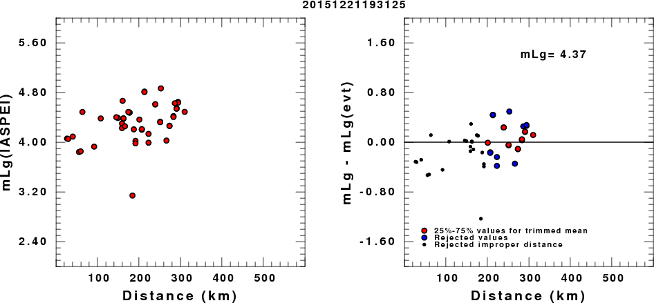
(a) mLg computed using the IASPEI formula; (b) mLg residuals ; the values used for the trimmed mean are indicated.
2015/12/21 19:31:25 36.03 126.96 10.0 3.9 Korea
USGS Felt map for this earthquake
 USGS/SLU Moment Tensor Solution
 ENS  2015/12/21 19:31:25:0  36.03  126.96  10.0 3.9 Korea

 Stations used:
   KS.BAR KS.BUS2 KS.DACB KS.DAG2 KS.DGY2 KS.HWCB KS.JJU
   KS.KOHB KS.SEHB KS.SEO2 KS.YNCB

 Filtering commands used:
   cut o DIST/3.3 -30 o DIST/3.3 +70
   rtr
   taper w 0.1
   hp c 0.02 n 3
   lp c 0.10 n 3

 Best Fitting Double Couple
  Mo = 9.55e+21 dyne-cm
  Mw = 3.92
  Z  = 9 km
  Plane   Strike  Dip  Rake
   NP1      201    54   110
   NP2      350    40    65
  Principal Axes:
   Axis    Value   Plunge  Azimuth
    T   9.55e+21     72     163
    N   0.00e+00     16      10
    P  -9.55e+21      7     278

 Moment Tensor: (dyne-cm)
    Component   Value
       Mxx     6.30e+20
       Mxy     9.80e+20
       Mxz    -2.78e+21
       Myy    -9.15e+21
       Myz     2.02e+21
       Mzz     8.52e+21


                     -------#######
                 ----------------------
              --------------#####---------
             -------------#########--------
           --------------###########---------
          -------------##############---------
         -------------################---------
        -------------##################---------
          ----------####################--------
        P ---------#####################---------
          ---------#####################---------
       -----------#######################--------
       -----------##########   ##########--------
        ----------########## T ##########-------
        ---------###########   #########--------
         --------#######################-------
          -------######################-------
           -------#####################------
             -----####################-----
              -----##################-----
                 --################----
                     ############--


 Global CMT Convention Moment Tensor:
      R          T          P
  8.52e+21  -2.78e+21  -2.02e+21
 -2.78e+21   6.30e+20  -9.80e+20
 -2.02e+21  -9.80e+20  -9.15e+21


Details of the solution is found at

http://www.eas.slu.edu/eqc/eqc_mt/MECH.NA/20151221193125/index.html
|
      STK = 350
      DIP = 40
     RAKE = 65
       MW = 3.92
       HS = 9.0
The NDK file is 20151221193125.ndk The waveform inversion is preferred.
The following compares this source inversion to others
 USGS/SLU Moment Tensor Solution
 ENS  2015/12/21 19:31:25:0  36.03  126.96  10.0 3.9 Korea

 Stations used:
   KS.BAR KS.BUS2 KS.DACB KS.DAG2 KS.DGY2 KS.HWCB KS.JJU
   KS.KOHB KS.SEHB KS.SEO2 KS.YNCB

 Filtering commands used:
   cut o DIST/3.3 -30 o DIST/3.3 +70
   rtr
   taper w 0.1
   hp c 0.02 n 3
   lp c 0.10 n 3

 Best Fitting Double Couple
  Mo = 9.55e+21 dyne-cm
  Mw = 3.92
  Z  = 9 km
  Plane   Strike  Dip  Rake
   NP1      201    54   110
   NP2      350    40    65
  Principal Axes:
   Axis    Value   Plunge  Azimuth
    T   9.55e+21     72     163
    N   0.00e+00     16      10
    P  -9.55e+21      7     278

 Moment Tensor: (dyne-cm)
    Component   Value
       Mxx     6.30e+20
       Mxy     9.80e+20
       Mxz    -2.78e+21
       Myy    -9.15e+21
       Myz     2.02e+21
       Mzz     8.52e+21


                     -------#######
                 ----------------------
              --------------#####---------
             -------------#########--------
           --------------###########---------
          -------------##############---------
         -------------################---------
        -------------##################---------
          ----------####################--------
        P ---------#####################---------
          ---------#####################---------
       -----------#######################--------
       -----------##########   ##########--------
        ----------########## T ##########-------
        ---------###########   #########--------
         --------#######################-------
          -------######################-------
           -------#####################------
             -----####################-----
              -----##################-----
                 --################----
                     ############--


 Global CMT Convention Moment Tensor:
      R          T          P
  8.52e+21  -2.78e+21  -2.02e+21
 -2.78e+21   6.30e+20  -9.80e+20
 -2.02e+21  -9.80e+20  -9.15e+21


Details of the solution is found at

http://www.eas.slu.edu/eqc/eqc_mt/MECH.NA/20151221193125/index.html
|
(a) mLg computed using the IASPEI formula; (b) mLg residuals ; the values used for the trimmed mean are indicated.
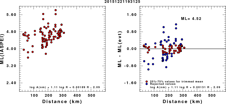
(a) ML computed using the IASPEI formula; (b) ML residuals computed using a modified IASPEI formula that accounts for path specific attenuation; the values used for the trimmed mean are indicated. The ML relation used for each figure is given at the bottom of each plot.
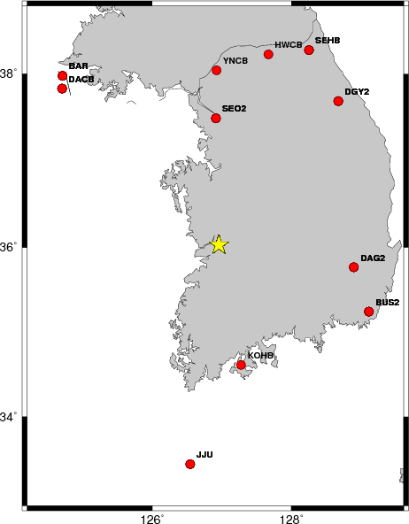
The focal mechanism was determined using broadband seismic waveforms. The location of the event and the and stations used for the waveform inversion are shown in the next figure.
|
|
|
The program wvfgrd96 was used with good traces observed at short distance to determine the focal mechanism, depth and seismic moment. This technique requires a high quality signal and well determined velocity model for the Green functions. To the extent that these are the quality data, this type of mechanism should be preferred over the radiation pattern technique which requires the separate step of defining the pressure and tension quadrants and the correct strike.
The observed and predicted traces are filtered using the following gsac commands:
cut o DIST/3.3 -30 o DIST/3.3 +70
rtr
taper w 0.1
hp c 0.02 n 3
lp c 0.10 n 3
The results of this grid search from 0.5 to 19 km depth are as follow:
           DEPTH  STK   DIP  RAKE   MW    FIT
WVFGRD96    1.0    85    30   -75   3.77 0.6116
WVFGRD96    2.0   295    25   -35   3.84 0.5973
WVFGRD96    3.0   300    25   -30   3.84 0.6357
WVFGRD96    4.0   310    30   -20   3.83 0.6646
WVFGRD96    5.0   320    35     0   3.82 0.6843
WVFGRD96    6.0   345    40    55   3.91 0.7333
WVFGRD96    7.0   350    40    65   3.93 0.7782
WVFGRD96    8.0   350    40    65   3.93 0.8006
WVFGRD96    9.0   350    40    65   3.92 0.8043
WVFGRD96   10.0   345    45    60   3.92 0.7976
WVFGRD96   11.0   345    45    60   3.92 0.7833
WVFGRD96   12.0   350    40    60   3.92 0.7641
WVFGRD96   13.0   340    45    50   3.92 0.7420
WVFGRD96   14.0   340    45    50   3.92 0.7173
WVFGRD96   15.0   340    45    50   3.93 0.6905
WVFGRD96   16.0   340    45    50   3.93 0.6623
WVFGRD96   17.0   340    45    45   3.94 0.6324
WVFGRD96   18.0   340    45    45   3.94 0.6035
WVFGRD96   19.0   340    45    45   3.95 0.5745
WVFGRD96   20.0   335    45    45   3.95 0.5462
WVFGRD96   21.0   335    45    40   3.96 0.5183
WVFGRD96   22.0   335    45    40   3.96 0.4921
WVFGRD96   23.0   335    45    40   3.97 0.4671
WVFGRD96   24.0   240    60    60   3.94 0.4473
WVFGRD96   25.0   240    60    60   3.95 0.4282
WVFGRD96    0.0****** 32767     1   0.00-2.0000
WVFGRD96    0.0****** 32767     1   0.00-2.0000
WVFGRD96    0.0****** 32767     1   0.00-2.0000
WVFGRD96    0.0****** 32767     1   0.00-2.0000
The best solution is
WVFGRD96 9.0 350 40 65 3.92 0.8043
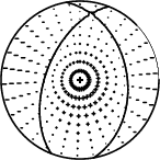
The mechanism correspond to the best fit is
|
|
|
The best fit as a function of depth is given in the following figure:
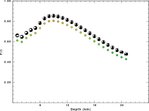
|
|
|
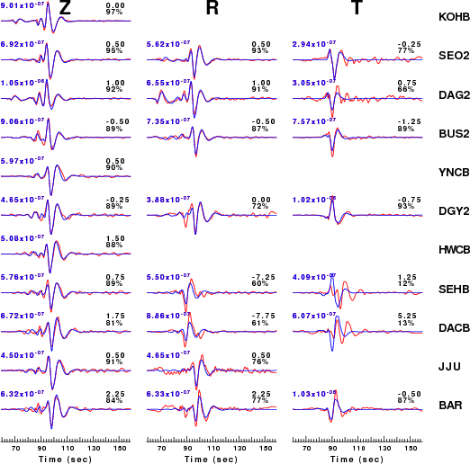
The comparison of the observed and predicted waveforms is given in the next figure. The red traces are the observed and the blue are the predicted. Each observed-predicted component is plotted to the same scale and peak amplitudes are indicated by the numbers to the left of each trace. A pair of numbers is given in black at the right of each predicted traces. The upper number it the time shift required for maximum correlation between the observed and predicted traces. This time shift is required because the synthetics are not computed at exactly the same distance as the observed and because the velocity model used in the predictions may not be perfect. A positive time shift indicates that the prediction is too fast and should be delayed to match the observed trace (shift to the right in this figure). A negative value indicates that the prediction is too slow. The lower number gives the percentage of variance reduction to characterize the individual goodness of fit (100% indicates a perfect fit).
The bandpass filter used in the processing and for the display was
cut o DIST/3.3 -30 o DIST/3.3 +70
rtr
taper w 0.1
hp c 0.02 n 3
lp c 0.10 n 3
|
|
|
|
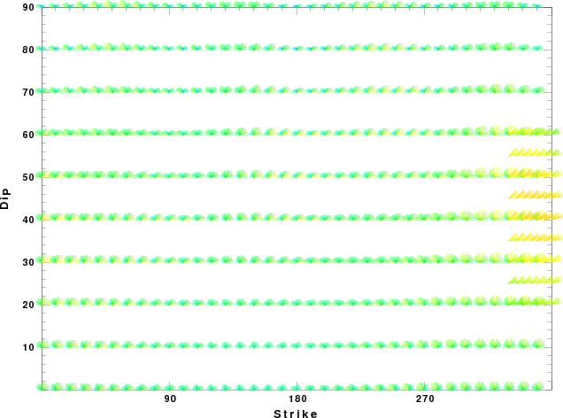
| Focal mechanism sensitivity at the preferred depth. The red color indicates a very good fit to thewavefroms. Each solution is plotted as a vector at a given value of strike and dip with the angle of the vector representing the rake angle, measured, with respect to the upward vertical (N) in the figure. |
A check on the assumed source location is possible by looking at the time shifts between the observed and predicted traces. The time shifts for waveform matching arise for several reasons:
Time_shift = A + B cos Azimuth + C Sin Azimuth
The time shifts for this inversion lead to the next figure:
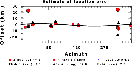
The derived shift in origin time and epicentral coordinates are given at the bottom of the figure.
Thanks also to the many seismic network operators whose dedication make this effort possible: University of Nevada Reno, University of Alaska, University of Washington, Oregon State University, University of Utah, Montana Bureas of Mines, UC Berkely, Caltech, UC San Diego, Saint Louis University, University of Memphis, Lamont Doherty Earth Observatory, the Iris stations and the Transportable Array of EarthScope.
The t6.invSNU.CUVEL.model was used for the waveform synthetic seismograms and for the surface wave eigenfunctions and dispersion is as follows:
MODEL.01
Model after    30 iterations
ISOTROPIC
KGS
SPHERICAL EARTH
1-D
CONSTANT VELOCITY
LINE08
LINE09
LINE10
LINE11
      H(KM)   VP(KM/S)   VS(KM/S) RHO(GM/CC)         QP         QS       ETAP       ETAS      FREFP      FREFS
     1.0000     5.3800     3.0009     2.5772  0.118E-02  0.167E-02   0.00       0.00       1.00       1.00
     1.0000     5.8057     3.2383     2.6606  0.118E-02  0.167E-02   0.00       0.00       1.00       1.00
     1.0000     6.1732     3.4433     2.7513  0.118E-02  0.167E-02   0.00       0.00       1.00       1.00
     3.0000     6.2872     3.5067     2.7862  0.118E-02  0.167E-02   0.00       0.00       1.00       1.00
     5.0000     6.3245     3.5281     2.7970  0.118E-02  0.167E-02   0.00       0.00       1.00       1.00
     5.0000     6.4165     3.5788     2.8248  0.118E-02  0.167E-02   0.00       0.00       1.00       1.00
     4.0000     6.5576     3.6576     2.8653  0.118E-02  0.167E-02   0.00       0.00       1.00       1.00
     5.0000     6.6402     3.7038     2.8865  0.118E-02  0.167E-02   0.00       0.00       1.00       1.00
     2.5000     6.6540     3.7115     2.8897  0.118E-02  0.167E-02   0.00       0.00       1.00       1.00
     2.5000     7.0960     3.9579     3.0111  0.118E-02  0.167E-02   0.00       0.00       1.00       1.00
     2.5000     7.9155     4.4148     3.2804  0.118E-02  0.167E-02   0.00       0.00       1.00       1.00
     2.5000     7.8925     4.4019     3.2735  0.118E-02  0.167E-02   0.00       0.00       1.00       1.00
     5.0000     7.8665     4.3876     3.2643  0.118E-02  0.167E-02   0.00       0.00       1.00       1.00
     5.0000     7.5675     4.2211     3.1625  0.118E-02  0.167E-02   0.00       0.00       1.00       1.00
     5.0000     7.7550     4.3252     3.2262  0.118E-02  0.167E-02   0.00       0.00       1.00       1.00
     5.0000     7.7602     4.3280     3.2282  0.118E-02  0.167E-02   0.00       0.00       1.00       1.00
     5.0000     7.7958     4.3487     3.2398  0.118E-02  0.167E-02   0.00       0.00       1.00       1.00
     5.0000     7.7415     4.3195     3.2217  0.118E-02  0.167E-02   0.00       0.00       1.00       1.00
     5.0000     7.6497     4.2688     3.1915  0.118E-02  0.167E-02   0.00       0.00       1.00       1.00
     5.0000     7.6408     4.2653     3.1889  0.118E-02  0.167E-02   0.00       0.00       1.00       1.00
     5.0000     7.6666     4.2716     3.1976  0.118E-02  0.167E-02   0.00       0.00       1.00       1.00
     5.0000     7.6699     4.2830     3.1986  0.118E-02  0.167E-02   0.00       0.00       1.00       1.00
     5.0000     7.6780     4.2885     3.2014  0.118E-02  0.167E-02   0.00       0.00       1.00       1.00
     5.0000     7.6816     4.2896     3.2028  0.118E-02  0.167E-02   0.00       0.00       1.00       1.00
     5.0000     7.6946     4.2996     3.2072  0.118E-02  0.167E-02   0.00       0.00       1.00       1.00
    10.0000     7.7349     4.3197     3.2208  0.118E-02  0.167E-02   0.00       0.00       1.00       1.00
    10.0000     7.7791     4.3484     3.2355  0.118E-02  0.167E-02   0.00       0.00       1.00       1.00
    10.0000     7.8331     4.3722     3.2536  0.862E-02  0.131E-01   0.00       0.00       1.00       1.00
    10.0000     7.8824     4.3863     3.2703  0.862E-02  0.131E-01   0.00       0.00       1.00       1.00
    10.0000     7.9360     4.4024     3.2883  0.855E-02  0.131E-01   0.00       0.00       1.00       1.00
    10.0000     7.9967     4.4237     3.3088  0.847E-02  0.131E-01   0.00       0.00       1.00       1.00
    10.0000     8.0529     4.4423     3.3289  0.847E-02  0.131E-01   0.00       0.00       1.00       1.00
    10.0000     8.1110     4.4603     3.3496  0.833E-02  0.130E-01   0.00       0.00       1.00       1.00
    10.0000     8.1762     4.4832     3.3728  0.826E-02  0.129E-01   0.00       0.00       1.00       1.00
    10.0000     8.2410     4.5054     3.3959  0.813E-02  0.128E-01   0.00       0.00       1.00       1.00
    10.0000     8.3022     4.5257     3.4176  0.806E-02  0.126E-01   0.00       0.00       1.00       1.00
    10.0000     8.3635     4.5514     3.4395  0.474E-02  0.746E-02   0.00       0.00       1.00       1.00
    10.0000     8.4257     4.5839     3.4617  0.472E-02  0.741E-02   0.00       0.00       1.00       1.00
    10.0000     8.4845     4.6145     3.4827  0.469E-02  0.741E-02   0.00       0.00       1.00       1.00
    10.0000     8.5403     4.6434     3.5020  0.467E-02  0.735E-02   0.00       0.00       1.00       1.00
    10.0000     8.5934     4.6708     3.5199  0.465E-02  0.735E-02   0.00       0.00       1.00       1.00
    10.0000     8.6436     4.6959     3.5369  0.463E-02  0.730E-02   0.00       0.00       1.00       1.00
    10.0000     8.6912     4.7194     3.5530  0.461E-02  0.730E-02   0.00       0.00       1.00       1.00
    10.0000     8.7365     4.7413     3.5684  0.459E-02  0.725E-02   0.00       0.00       1.00       1.00
    10.0000     8.7797     4.7622     3.5831  0.455E-02  0.725E-02   0.00       0.00       1.00       1.00
    10.0000     8.8199     4.7819     3.5967  0.452E-02  0.719E-02   0.00       0.00       1.00       1.00
    10.0000     8.8587     4.8001     3.6099  0.450E-02  0.714E-02   0.00       0.00       1.00       1.00
    10.0000     8.8958     4.8177     3.6226  0.448E-02  0.714E-02   0.00       0.00       1.00       1.00
    10.0000     8.9314     4.8346     3.6347  0.446E-02  0.709E-02   0.00       0.00       1.00       1.00
    10.0000     8.9647     4.8500     3.6461  0.442E-02  0.704E-02   0.00       0.00       1.00       1.00
    10.0000     8.9962     4.8651     3.6569  0.441E-02  0.704E-02   0.00       0.00       1.00       1.00
    10.0000     9.0263     4.8783     3.6685  0.439E-02  0.699E-02   0.00       0.00       1.00       1.00
    10.0000     9.0547     4.8915     3.6800  0.435E-02  0.694E-02   0.00       0.00       1.00       1.00
    10.0000     9.0822     4.9041     3.6911  0.433E-02  0.690E-02   0.00       0.00       1.00       1.00
    10.0000     9.1091     4.9164     3.7020  0.431E-02  0.690E-02   0.00       0.00       1.00       1.00
    10.0000     9.1346     4.9280     3.7123  0.427E-02  0.685E-02   0.00       0.00       1.00       1.00
    10.0000     9.4876     5.1513     3.8537  0.388E-02  0.613E-02   0.00       0.00       1.00       1.00
    10.0000     9.5095     5.1663     3.8624  0.388E-02  0.613E-02   0.00       0.00       1.00       1.00
    10.0000     9.5299     5.1806     3.8703  0.386E-02  0.610E-02   0.00       0.00       1.00       1.00
    10.0000     9.5507     5.1944     3.8784  0.386E-02  0.610E-02   0.00       0.00       1.00       1.00
    10.0000     9.5706     5.2080     3.8861  0.385E-02  0.606E-02   0.00       0.00       1.00       1.00
    10.0000     9.5900     5.2214     3.8937  0.385E-02  0.606E-02   0.00       0.00       1.00       1.00
    10.0000     9.6090     5.2347     3.9011  0.383E-02  0.606E-02   0.00       0.00       1.00       1.00
    10.0000     9.6272     5.2480     3.9081  0.383E-02  0.602E-02   0.00       0.00       1.00       1.00
    10.0000     9.6458     5.2604     3.9154  0.383E-02  0.602E-02   0.00       0.00       1.00       1.00
    10.0000     9.6794     5.2816     3.9282  0.382E-02  0.599E-02   0.00       0.00       1.00       1.00
    10.0000     9.7130     5.3029     3.9409  0.382E-02  0.599E-02   0.00       0.00       1.00       1.00
    10.0000     9.7466     5.3242     3.9537  0.380E-02  0.599E-02   0.00       0.00       1.00       1.00
    10.0000     9.7799     5.3454     3.9664  0.380E-02  0.595E-02   0.00       0.00       1.00       1.00
    10.0000     9.8137     5.3669     3.9792  0.380E-02  0.595E-02   0.00       0.00       1.00       1.00
    10.0000     9.8473     5.3883     3.9920  0.379E-02  0.592E-02   0.00       0.00       1.00       1.00
    10.0000     9.8808     5.4094     4.0047  0.379E-02  0.592E-02   0.00       0.00       1.00       1.00
     0.0000     9.9144     5.4306     4.0175  0.377E-02  0.592E-02   0.00       0.00       1.00       1.00
Here we tabulate the reasons for not using certain digital data sets
The following stations did not have a valid response files: