2011/06/17 16:38:31 4.1 37.91 N 124.5 E
2011/06/17 07:38:33 37.886 124.787 9.5 4.2 Korea
 SLU Moment Tensor Solution
 2011/06/17 07:38:33 37.886 124.787 9.5 4.2 Korea

 Best Fitting Double Couple
    Mo = 7.24e+21 dyne-cm
    Mw = 3.84
    Z  = 16 km
     Plane   Strike  Dip  Rake
      NP1      115    80   -15
      NP2      208    75   -170
 Principal Axes:
   Axis    Value   Plunge  Azimuth
     T   7.24e+21      3     162
     N   0.00e+00     72     262
     P  -7.24e+21     18      71


 Moment Tensor: (dyne-cm)
    Component  Value
       Mxx     5.81e+21
       Mxy    -4.18e+21
       Mxz    -1.08e+21
       Myy    -5.16e+21
       Myz    -1.85e+21
       Mzz    -6.41e+20


                     ##############
                 ####################--
              ####################--------
             ####################----------
           ####################--------------
          ####################----------------
         -###################--------------   -
        ----###############---------------- P --
        ------############-----------------   --
       ----------########------------------------
       --------------###-------------------------
       ----------------#-------------------------
       ---------------######---------------------
        --------------##########----------------
        -------------################-----------
         -----------########################---
          ----------##########################
           --------##########################
             ------########################
              -----#######################
                 -###############   ###
                     ############ T


 Harvard Convention
 Moment Tensor:
      R          T          F
 -6.41e+20  -1.08e+21   1.85e+21
 -1.08e+21   5.81e+21   4.18e+21
  1.85e+21   4.18e+21  -5.16e+21


Details of the solution is found at

http://www.eas.slu.edu/eqc/eqc_mt/MECH.KR/20110617073833/index.html
|
      STK = 115
      DIP = 80
     RAKE = -15
       MW = 3.84
       HS = 16.0
The waveform inversion is preferred.
The following compares this source inversion to others
 SLU Moment Tensor Solution
 2011/06/17 07:38:33 37.886 124.787 9.5 4.2 Korea

 Best Fitting Double Couple
    Mo = 7.24e+21 dyne-cm
    Mw = 3.84
    Z  = 16 km
     Plane   Strike  Dip  Rake
      NP1      115    80   -15
      NP2      208    75   -170
 Principal Axes:
   Axis    Value   Plunge  Azimuth
     T   7.24e+21      3     162
     N   0.00e+00     72     262
     P  -7.24e+21     18      71


 Moment Tensor: (dyne-cm)
    Component  Value
       Mxx     5.81e+21
       Mxy    -4.18e+21
       Mxz    -1.08e+21
       Myy    -5.16e+21
       Myz    -1.85e+21
       Mzz    -6.41e+20


                     ##############
                 ####################--
              ####################--------
             ####################----------
           ####################--------------
          ####################----------------
         -###################--------------   -
        ----###############---------------- P --
        ------############-----------------   --
       ----------########------------------------
       --------------###-------------------------
       ----------------#-------------------------
       ---------------######---------------------
        --------------##########----------------
        -------------################-----------
         -----------########################---
          ----------##########################
           --------##########################
             ------########################
              -----#######################
                 -###############   ###
                     ############ T


 Harvard Convention
 Moment Tensor:
      R          T          F
 -6.41e+20  -1.08e+21   1.85e+21
 -1.08e+21   5.81e+21   4.18e+21
  1.85e+21   4.18e+21  -5.16e+21


Details of the solution is found at

http://www.eas.slu.edu/Earthquake_Center/MECH.KR/20110617073833/index.html
|
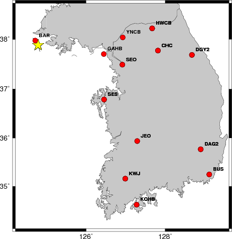
The focal mechanism was determined using broadband seismic waveforms. The location of the event and the and stations used for the waveform inversion are shown in the next figure.
|
|
|
|
The program wvfgrd96 was used with good traces observed at short distance to determine the focal mechanism, depth and seismic moment. This technique requires a high quality signal and well determined velocity model for the Green functions. To the extent that these are the quality data, this type of mechanism should be preferred over the radiation pattern technique which requires the separate step of defining the pressure and tension quadrants and the correct strike.
The observed and predicted traces are filtered using the following gsac commands:
hp c 0.02 n 3
lp c 0.10 n 3
The results of this grid search from 0.5 to 19 km depth are as follow:
           DEPTH  STK   DIP  RAKE   MW    FIT
WVFGRD96    0.5   210    75    10   3.53 0.4958
WVFGRD96    1.0   210    80    15   3.55 0.5031
WVFGRD96    2.0   295    80    10   3.61 0.5077
WVFGRD96    3.0   305    60    40   3.69 0.5462
WVFGRD96    4.0   300    70    25   3.67 0.5680
WVFGRD96    5.0   110    70   -25   3.68 0.6017
WVFGRD96    6.0   110    70   -20   3.68 0.6322
WVFGRD96    7.0   110    70   -20   3.69 0.6559
WVFGRD96    8.0   110    70   -15   3.70 0.6764
WVFGRD96    9.0   110    70   -15   3.71 0.6944
WVFGRD96   10.0   115    75   -15   3.74 0.7095
WVFGRD96   11.0   115    75   -15   3.75 0.7239
WVFGRD96   12.0   115    75   -15   3.77 0.7366
WVFGRD96   13.0   115    75   -10   3.79 0.7456
WVFGRD96   14.0   115    75   -10   3.81 0.7536
WVFGRD96   15.0   115    80   -10   3.82 0.7595
WVFGRD96   16.0   115    80   -15   3.84 0.7644
WVFGRD96   17.0   115    80   -15   3.86 0.7636
WVFGRD96   18.0   115    80   -15   3.88 0.7608
WVFGRD96   19.0   115    80   -15   3.89 0.7560
WVFGRD96   20.0   115    80   -15   3.91 0.7462
WVFGRD96   21.0   115    85   -15   3.92 0.7372
WVFGRD96   22.0   115    85   -15   3.93 0.7263
WVFGRD96   23.0   295    90     5   3.94 0.7044
WVFGRD96   24.0   115    85   -15   3.96 0.6963
WVFGRD96   25.0   295    90    10   3.97 0.6734
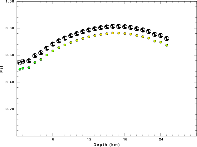
The best solution is
WVFGRD96 16.0 115 80 -15 3.84 0.7644
The mechanism correspond to the best fit is
|
|
|
The best fit as a function of depth is given in the following figure:
|
|
|
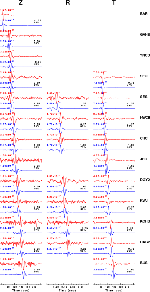
The comparison of the observed and predicted waveforms is given in the next figure. The red traces are the observed and the blue are the predicted. Each observed-predicted component is plotted to the same scale and peak amplitudes are indicated by the numbers to the left of each trace. A pair of numbers is given in black at the right of each predicted traces. The upper number it the time shift required for maximum correlation between the observed and predicted traces. This time shift is required because the synthetics are not computed at exactly the same distance as the observed and because the velocity model used in the predictions may not be perfect. A positive time shift indicates that the prediction is too fast and should be delayed to match the observed trace (shift to the right in this figure). A negative value indicates that the prediction is too slow. The lower number gives the percentage of variance reduction to characterize the individual goodness of fit (100% indicates a perfect fit).
The bandpass filter used in the processing and for the display was
hp c 0.02 n 3
lp c 0.10 n 3
|
|
|
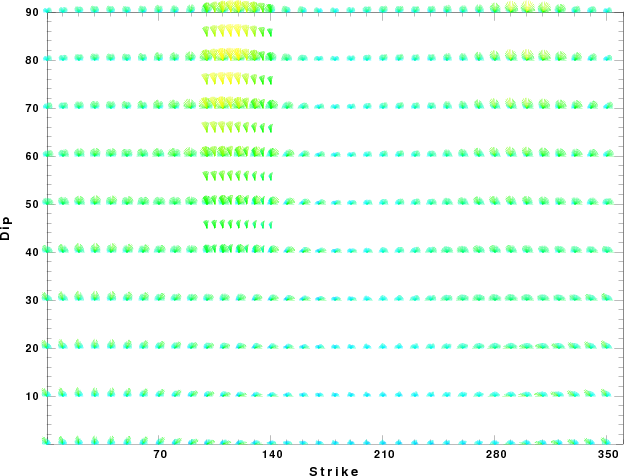
|
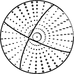
| Focal mechanism sensitivity at the preferred depth. The red color indicates a very good fit to thewavefroms. Each solution is plotted as a vector at a given value of strike and dip with the angle of the vector representing the rake angle, measured, with respect to the upward vertical (N) in the figure. |
A check on the assumed source location is possible by looking at the time shifts between the observed and predicted traces. The time shifts for waveform matching arise for several reasons:
Time_shift = A + B cos Azimuth + C Sin Azimuth
The time shifts for this inversion lead to the next figure:
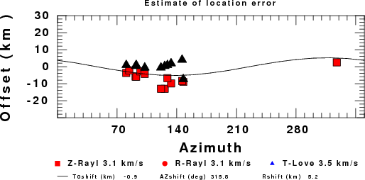
The derived shift in origin time and epicentral coordinates are given at the bottom of the figure.
The t6.invSNU.CUVEL used for the waveform synthetic seismograms and for the surface wave eigenfunctions and dispersion is as follows:
MODEL.01
Model after    30 iterations
ISOTROPIC
KGS
SPHERICAL EARTH
1-D
CONSTANT VELOCITY
LINE08
LINE09
LINE10
LINE11
      H(KM)   VP(KM/S)   VS(KM/S) RHO(GM/CC)         QP         QS       ETAP       ETAS      FREFP      FREFS
     1.0000     5.3800     3.0009     2.5772  0.118E-02  0.167E-02   0.00       0.00       1.00       1.00
     1.0000     5.8057     3.2383     2.6606  0.118E-02  0.167E-02   0.00       0.00       1.00       1.00
     1.0000     6.1732     3.4433     2.7513  0.118E-02  0.167E-02   0.00       0.00       1.00       1.00
     3.0000     6.2872     3.5067     2.7862  0.118E-02  0.167E-02   0.00       0.00       1.00       1.00
     5.0000     6.3245     3.5281     2.7970  0.118E-02  0.167E-02   0.00       0.00       1.00       1.00
     5.0000     6.4165     3.5788     2.8248  0.118E-02  0.167E-02   0.00       0.00       1.00       1.00
     4.0000     6.5576     3.6576     2.8653  0.118E-02  0.167E-02   0.00       0.00       1.00       1.00
     5.0000     6.6402     3.7038     2.8865  0.118E-02  0.167E-02   0.00       0.00       1.00       1.00
     2.5000     6.6540     3.7115     2.8897  0.118E-02  0.167E-02   0.00       0.00       1.00       1.00
     2.5000     7.0960     3.9579     3.0111  0.118E-02  0.167E-02   0.00       0.00       1.00       1.00
     2.5000     7.9155     4.4148     3.2804  0.118E-02  0.167E-02   0.00       0.00       1.00       1.00
     2.5000     7.8925     4.4019     3.2735  0.118E-02  0.167E-02   0.00       0.00       1.00       1.00
     5.0000     7.8665     4.3876     3.2643  0.118E-02  0.167E-02   0.00       0.00       1.00       1.00
     5.0000     7.5675     4.2211     3.1625  0.118E-02  0.167E-02   0.00       0.00       1.00       1.00
     5.0000     7.7550     4.3252     3.2262  0.118E-02  0.167E-02   0.00       0.00       1.00       1.00
     5.0000     7.7602     4.3280     3.2282  0.118E-02  0.167E-02   0.00       0.00       1.00       1.00
     5.0000     7.7958     4.3487     3.2398  0.118E-02  0.167E-02   0.00       0.00       1.00       1.00
     5.0000     7.7415     4.3195     3.2217  0.118E-02  0.167E-02   0.00       0.00       1.00       1.00
     5.0000     7.6497     4.2688     3.1915  0.118E-02  0.167E-02   0.00       0.00       1.00       1.00
     5.0000     7.6408     4.2653     3.1889  0.118E-02  0.167E-02   0.00       0.00       1.00       1.00
     5.0000     7.6666     4.2716     3.1976  0.118E-02  0.167E-02   0.00       0.00       1.00       1.00
     5.0000     7.6699     4.2830     3.1986  0.118E-02  0.167E-02   0.00       0.00       1.00       1.00
     5.0000     7.6780     4.2885     3.2014  0.118E-02  0.167E-02   0.00       0.00       1.00       1.00
     5.0000     7.6816     4.2896     3.2028  0.118E-02  0.167E-02   0.00       0.00       1.00       1.00
     5.0000     7.6946     4.2996     3.2072  0.118E-02  0.167E-02   0.00       0.00       1.00       1.00
    10.0000     7.7349     4.3197     3.2208  0.118E-02  0.167E-02   0.00       0.00       1.00       1.00
    10.0000     7.7791     4.3484     3.2355  0.118E-02  0.167E-02   0.00       0.00       1.00       1.00
    10.0000     7.8331     4.3722     3.2536  0.862E-02  0.131E-01   0.00       0.00       1.00       1.00
    10.0000     7.8824     4.3863     3.2703  0.862E-02  0.131E-01   0.00       0.00       1.00       1.00
    10.0000     7.9360     4.4024     3.2883  0.855E-02  0.131E-01   0.00       0.00       1.00       1.00
    10.0000     7.9967     4.4237     3.3088  0.847E-02  0.131E-01   0.00       0.00       1.00       1.00
    10.0000     8.0529     4.4423     3.3289  0.847E-02  0.131E-01   0.00       0.00       1.00       1.00
    10.0000     8.1110     4.4603     3.3496  0.833E-02  0.130E-01   0.00       0.00       1.00       1.00
    10.0000     8.1762     4.4832     3.3728  0.826E-02  0.129E-01   0.00       0.00       1.00       1.00
    10.0000     8.2410     4.5054     3.3959  0.813E-02  0.128E-01   0.00       0.00       1.00       1.00
    10.0000     8.3022     4.5257     3.4176  0.806E-02  0.126E-01   0.00       0.00       1.00       1.00
    10.0000     8.3635     4.5514     3.4395  0.474E-02  0.746E-02   0.00       0.00       1.00       1.00
    10.0000     8.4257     4.5839     3.4617  0.472E-02  0.741E-02   0.00       0.00       1.00       1.00
    10.0000     8.4845     4.6145     3.4827  0.469E-02  0.741E-02   0.00       0.00       1.00       1.00
    10.0000     8.5403     4.6434     3.5020  0.467E-02  0.735E-02   0.00       0.00       1.00       1.00
    10.0000     8.5934     4.6708     3.5199  0.465E-02  0.735E-02   0.00       0.00       1.00       1.00
    10.0000     8.6436     4.6959     3.5369  0.463E-02  0.730E-02   0.00       0.00       1.00       1.00
    10.0000     8.6912     4.7194     3.5530  0.461E-02  0.730E-02   0.00       0.00       1.00       1.00
    10.0000     8.7365     4.7413     3.5684  0.459E-02  0.725E-02   0.00       0.00       1.00       1.00
    10.0000     8.7797     4.7622     3.5831  0.455E-02  0.725E-02   0.00       0.00       1.00       1.00
    10.0000     8.8199     4.7819     3.5967  0.452E-02  0.719E-02   0.00       0.00       1.00       1.00
    10.0000     8.8587     4.8001     3.6099  0.450E-02  0.714E-02   0.00       0.00       1.00       1.00
    10.0000     8.8958     4.8177     3.6226  0.448E-02  0.714E-02   0.00       0.00       1.00       1.00
    10.0000     8.9314     4.8346     3.6347  0.446E-02  0.709E-02   0.00       0.00       1.00       1.00
    10.0000     8.9647     4.8500     3.6461  0.442E-02  0.704E-02   0.00       0.00       1.00       1.00
    10.0000     8.9962     4.8651     3.6569  0.441E-02  0.704E-02   0.00       0.00       1.00       1.00
    10.0000     9.0263     4.8783     3.6685  0.439E-02  0.699E-02   0.00       0.00       1.00       1.00
    10.0000     9.0547     4.8915     3.6800  0.435E-02  0.694E-02   0.00       0.00       1.00       1.00
    10.0000     9.0822     4.9041     3.6911  0.433E-02  0.690E-02   0.00       0.00       1.00       1.00
    10.0000     9.1091     4.9164     3.7020  0.431E-02  0.690E-02   0.00       0.00       1.00       1.00
    10.0000     9.1346     4.9280     3.7123  0.427E-02  0.685E-02   0.00       0.00       1.00       1.00
    10.0000     9.4876     5.1513     3.8537  0.388E-02  0.613E-02   0.00       0.00       1.00       1.00
    10.0000     9.5095     5.1663     3.8624  0.388E-02  0.613E-02   0.00       0.00       1.00       1.00
    10.0000     9.5299     5.1806     3.8703  0.386E-02  0.610E-02   0.00       0.00       1.00       1.00
    10.0000     9.5507     5.1944     3.8784  0.386E-02  0.610E-02   0.00       0.00       1.00       1.00
    10.0000     9.5706     5.2080     3.8861  0.385E-02  0.606E-02   0.00       0.00       1.00       1.00
    10.0000     9.5900     5.2214     3.8937  0.385E-02  0.606E-02   0.00       0.00       1.00       1.00
    10.0000     9.6090     5.2347     3.9011  0.383E-02  0.606E-02   0.00       0.00       1.00       1.00
    10.0000     9.6272     5.2480     3.9081  0.383E-02  0.602E-02   0.00       0.00       1.00       1.00
    10.0000     9.6458     5.2604     3.9154  0.383E-02  0.602E-02   0.00       0.00       1.00       1.00
    10.0000     9.6794     5.2816     3.9282  0.382E-02  0.599E-02   0.00       0.00       1.00       1.00
    10.0000     9.7130     5.3029     3.9409  0.382E-02  0.599E-02   0.00       0.00       1.00       1.00
    10.0000     9.7466     5.3242     3.9537  0.380E-02  0.599E-02   0.00       0.00       1.00       1.00
    10.0000     9.7799     5.3454     3.9664  0.380E-02  0.595E-02   0.00       0.00       1.00       1.00
    10.0000     9.8137     5.3669     3.9792  0.380E-02  0.595E-02   0.00       0.00       1.00       1.00
    10.0000     9.8473     5.3883     3.9920  0.379E-02  0.592E-02   0.00       0.00       1.00       1.00
    10.0000     9.8808     5.4094     4.0047  0.379E-02  0.592E-02   0.00       0.00       1.00       1.00
     0.0000     9.9144     5.4306     4.0175  0.377E-02  0.592E-02   0.00       0.00       1.00       1.00
DATE=Fri Jun 24 01:24:29 CDT 2011