Location
2009/05/01 22:58:28 36.56 128.71 9.0 3.8 Korea
After the initial inversion run, I noticed that large time shifts were required to fit the wavesforms. These were approximately -3.5 sec for JJU, -3.25 for KWJ, -0.5 for CHC, -2.75 for DAGbut only 0.5 for CHJ. Since these were not all the same, and since I have confidence in my velocity model, an event mislocation is possible. I then went to the KMA pages http://www.kma.go.kr/neis/neis_02_02_03.jsp to get the coordinates of the accelerometer channels and http://www.kma.go.kr/neis/neis_02_02_02.jsp to get the coordinates of the short-period abd broadband velocity channels. At a few stations, there were some differences in the station name and coordinates in the two data sets. Hopefully KMA uses a station code internally to distinguish the channels.
I then picked P-wave first arrivals from all of the vertical traces. At some stations, it was possible to see the low-frequency Pn pull out from the Pg, which is expected from theory if the Moho is a sharp velocity discontinuity. The arrivals were then input to the program elocate. The complete run of the program is contained in the file elocate_out.txt. The arrival time data file for elocate is elocate.dat and the VEL.MOD file which contains my Korea velocity model in modified HYPO71 format at the bottom (modified since P S and Lg are defined and the number in the left column is the depth in km tp the top of the layer) is in the file VEL.MOD. The time shifts seen in the solution were reduced by about 1 second at the larger distances. Of course do not worry about the station JJU which has a partial path through the sea.
Evetn after this effort, the time shifts are negative which indicates that the model used to generate the Green's functions is somewhat slow. In another test, I removed the station ADO which has very different coordinates on the KMA pages; rmoving this station only affected the source depth.
The location used in the inversion is that of my relocation:
 Error Ellipse  X=   0.3493 km  Y= 0.3895 km  Theta = 157.4272 deg

 RMS Error        :               0.123              sec
 Travel_Time_Table:          KOREA
 Latitude         :             36.5588 +-    0.0032 N         0.3555 km
 Longitude        :            128.7133 +-    0.0043 E         0.3838 km
 Depth            :                9.07 +-      1.13 km
 Epoch Time       :      1241218708.649 +-      0.04 sec
 Event Time       :  20090501225828.649 +-      0.04 sec
 HYPO71 Quality   :                  CA
 Gap              :                  29              deg
Focal Mechanism
 SLU Moment Tensor Solution
 2009/05/01 22:58:28 36.56 128.71 9.0 3.8 Korea

 Best Fitting Double Couple
    Mo = 4.47e+21 dyne-cm
    Mw = 3.70
    Z  = 10 km
     Plane   Strike  Dip  Rake
      NP1      305    75    40
      NP2      203    52   161
 Principal Axes:
   Axis    Value   Plunge  Azimuth
     T   4.47e+21     38     171
     N   0.00e+00     48     322
     P  -4.47e+21     15      69


 Moment Tensor: (dyne-cm)
    Component  Value
       Mxx     2.14e+21
       Mxy    -1.80e+21
       Mxz    -2.54e+21
       Myy    -3.58e+21
       Myz    -7.01e+20
       Mzz     1.44e+21


                     ##############
                 ##############--------
              ##############--------------
             #############-----------------
           #############---------------------
          -------######-----------------------
         ------------#---------------------   -
        ------------#####------------------ P --
        -----------#########---------------   --
       ------------############------------------
       -----------###############----------------
       -----------#################--------------
       ----------#####################-----------
        ---------######################---------
        ---------########################-------
         --------##########################----
          -------###########   #############--
           ------########### T ##############
             -----##########   ############
              ----########################
                 --####################
                     ##############


 Harvard Convention
 Moment Tensor:
      R          T          F
  1.44e+21  -2.54e+21   7.01e+20
 -2.54e+21   2.14e+21   1.80e+21
  7.01e+20   1.80e+21  -3.58e+21


Details of the solution is found at

http://www.eas.slu.edu/eqc/eqc_mt/MECH.KR/20090501225828/index.html
|
Preferred Solution
The preferred solution from an analysis of the surface-wave spectral amplitude radiation pattern, waveform inversion and first motion observations is
      STK = 305
      DIP = 75
     RAKE = 40
       MW = 3.70
       HS = 10.0
The waveform inversion is preferred.
Moment Tensor Comparison
The following compares this source inversion to others
| SLU |
PWAVE |
 SLU Moment Tensor Solution
 2009/05/01 22:58:28 36.56 128.71 9.0 3.8 Korea

 Best Fitting Double Couple
    Mo = 4.47e+21 dyne-cm
    Mw = 3.70
    Z  = 10 km
     Plane   Strike  Dip  Rake
      NP1      305    75    40
      NP2      203    52   161
 Principal Axes:
   Axis    Value   Plunge  Azimuth
     T   4.47e+21     38     171
     N   0.00e+00     48     322
     P  -4.47e+21     15      69


 Moment Tensor: (dyne-cm)
    Component  Value
       Mxx     2.14e+21
       Mxy    -1.80e+21
       Mxz    -2.54e+21
       Myy    -3.58e+21
       Myz    -7.01e+20
       Mzz     1.44e+21


                     ##############
                 ##############--------
              ##############--------------
             #############-----------------
           #############---------------------
          -------######-----------------------
         ------------#---------------------   -
        ------------#####------------------ P --
        -----------#########---------------   --
       ------------############------------------
       -----------###############----------------
       -----------#################--------------
       ----------#####################-----------
        ---------######################---------
        ---------########################-------
         --------##########################----
          -------###########   #############--
           ------########### T ##############
             -----##########   ############
              ----########################
                 --####################
                     ##############


 Harvard Convention
 Moment Tensor:
      R          T          F
  1.44e+21  -2.54e+21   7.01e+20
 -2.54e+21   2.14e+21   1.80e+21
  7.01e+20   1.80e+21  -3.58e+21


Details of the solution is found at

http://www.eas.slu.edu/Earthquake_Center/MECH.KR/20090501225828/index.html
|
P-wave first motion data and waveform nodal planes
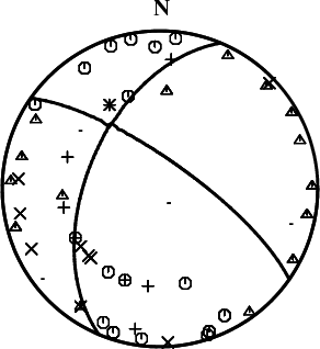
The circle and triangle indicate strong compressions and dilatations, respectively. The + and - indicate weak compressions and dilatations, respectively. The X indicates an arrival with indiscernible polarity due to prro signal-to-noise
|
Waveform Inversion
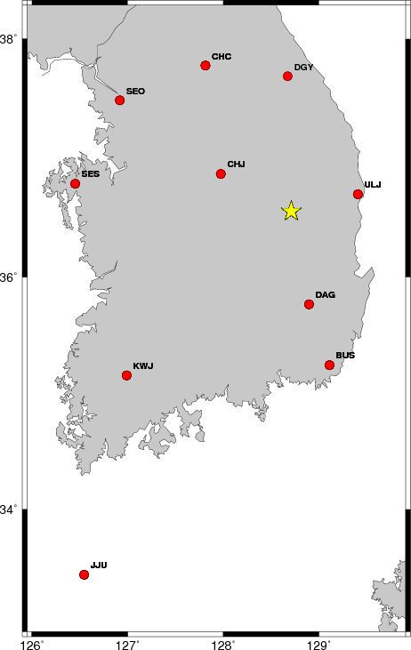
The focal mechanism was determined using broadband seismic waveforms. The location of the event and the
and stations used for the waveform inversion are shown in the next figure.
|
|
Location of broadband stations used for waveform inversion
|
The program wvfgrd96 was used with good traces observed at short distance to determine the focal mechanism, depth and seismic moment. This technique requires a high quality signal and well determined velocity model for the Green functions. To the extent that these are the quality data, this type of mechanism should be preferred over the radiation pattern technique which requires the separate step of defining the pressure and tension quadrants and the correct strike.
The observed and predicted traces are filtered using the following gsac commands:
hp c 0.02 n 3
lp c 0.10 n 3
The results of this grid search from 0.5 to 19 km depth are as follow:
           DEPTH  STK   DIP  RAKE   MW    FIT
WVFGRD96    0.5   295    90     0   3.49 0.6285
WVFGRD96    1.0   295    90     0   3.52 0.6449
WVFGRD96    2.0   115    85   -40   3.61 0.6576
WVFGRD96    3.0   115    85   -45   3.64 0.6930
WVFGRD96    4.0   300    85    45   3.65 0.7269
WVFGRD96    5.0   300    85    40   3.66 0.7629
WVFGRD96    6.0   305    75    40   3.67 0.7882
WVFGRD96    7.0   305    75    40   3.67 0.8120
WVFGRD96    8.0   305    75    40   3.68 0.8286
WVFGRD96    9.0   305    75    40   3.69 0.8386
WVFGRD96   10.0   305    75    40   3.70 0.8422
WVFGRD96   11.0   305    75    35   3.71 0.8415
WVFGRD96   12.0   305    75    40   3.72 0.8405
WVFGRD96   13.0   305    75    40   3.73 0.8333
WVFGRD96   14.0   305    75    40   3.74 0.8239
WVFGRD96   15.0   305    75    40   3.74 0.8119
WVFGRD96   16.0   305    75    35   3.75 0.7969
WVFGRD96   17.0   305    75    40   3.77 0.7827
WVFGRD96   18.0   305    75    40   3.77 0.7641
WVFGRD96   19.0   305    75    40   3.78 0.7434
WVFGRD96   20.0   305    75    40   3.79 0.7201
WVFGRD96   21.0   305    75    40   3.80 0.6964
WVFGRD96   22.0   305    75    40   3.80 0.6703
WVFGRD96   23.0   305    75    40   3.80 0.6427
WVFGRD96   24.0   300    85    40   3.81 0.6173
WVFGRD96   25.0   300    85    40   3.81 0.5945
The best solution is
WVFGRD96 10.0 305 75 40 3.70 0.8422
The mechanism correspond to the best fit is
|
|
Figure 1. Waveform inversion focal mechanism
|
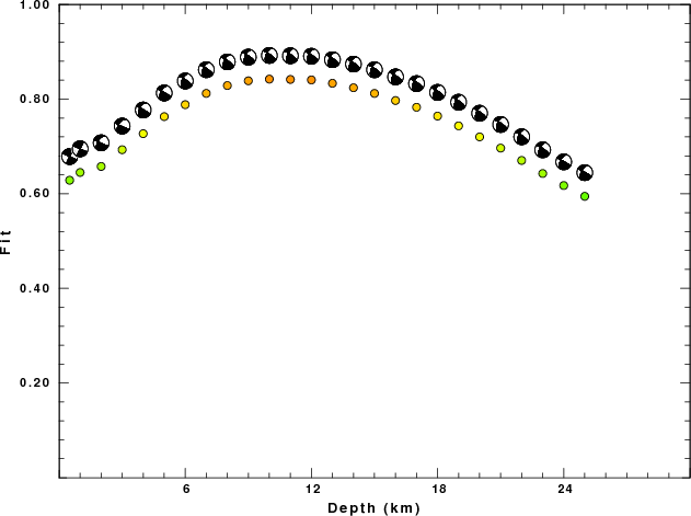
The best fit as a function of depth is given in the following figure:
|
|
Figure 2. Depth sensitivity for waveform mechanism
|
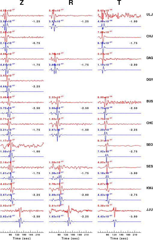
The comparison of the observed and predicted waveforms is given in the next figure. The red traces are the observed and the blue are the predicted.
Each observed-predicted componnet is plotted to the same scale and peak amplitudes are indicated by the numbers to the left of each trace. The number in black at the rightr of each predicted traces it the time shift required for maximum correlation between the observed and predicted traces. This time shift is required because the synthetics are not computed at exactly the same distance as the observed and because the velocity model used in the predictions may not be perfect.
A positive time shift indicates that the prediction is too fast and should be delayed to match the observed trace (shift to the right in this figure). A negative value indicates that the prediction is too slow.
The bandpass filter used in the processing and for the display was
hp c 0.02 n 3
lp c 0.10 n 3
|
|
Figure 3. Waveform comparison for selected depth
|
|
|
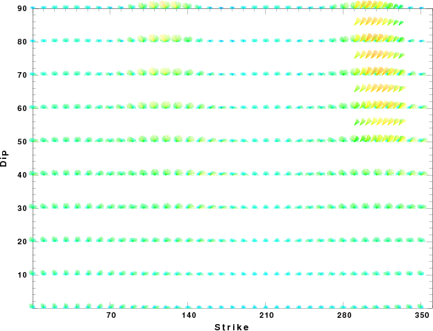
Focal mechanism sensitivity at the preferred depth. The red color indicates a very good fit to thewavefroms.
Each solution is plotted as a vector at a given value of strike and dip with the angle of the vector representing the rake angle, measured, with respect to the upward vertical (N) in the figure.
|
Surface-Wave Focal Mechanism
The following figure shows the stations used in the grid search for the best focal mechanism to fit the surface-wave spectral amplitudes of the Love and Rayleigh waves.

|
|
Location of broadband stations used to obtain focal mechanism from surface-wave spectral amplitudes
|
The surface-wave determined focal mechanism is shown here.
First motion data
The P-wave first motion data for focal mechanism studies are as follow:
Sta Az Dist First motion
Surface-wave analysis
Surface wave analysis was performed using codes from
Computer Programs in Seismology, specifically the
multiple filter analysis program do_mft and the surface-wave
radiation pattern search program srfgrd96.
Data preparation
Digital data were collected, instrument response removed and traces converted
to Z, R an T components. Multiple filter analysis was applied to the Z and T traces to obtain the Rayleigh- and Love-wave spectral amplitudes, respectively.
These were input to the search program which examined all depths between 1 and 25 km
and all possible mechanisms.

|
|
Best mechanism fit as a function of depth. The preferred depth is given above. Lower hemisphere projection
|

|
|
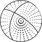
Pressure-tension axis trends. Since the surface-wave spectra search does not distinguish between P and T axes and since there is a 180 ambiguity in strike, all possible P and T axes are plotted. First motion data and waveforms will be used to select the preferred mechanism. The purpose of this plot is to provide an idea of the
possible range of solutions. The P and T-axes for all mechanisms with goodness of fit greater than 0.9 FITMAX (above) are plotted here.
|

|
|
Focal mechanism sensitivity at the preferred depth. The red color indicates a very good fit to the Love and Rayleigh wave radiation patterns.
Each solution is plotted as a vector at a given value of strike and dip with the angle of the vector representing the rake angle, measured, with respect to the upward vertical (N) in the figure. Because of the symmetry of the spectral amplitude rediation patterns, only strikes from 0-180 degrees are sampled.
|
Love-wave radiation patterns
Rayleigh-wave radiation patterns
Broadband station distribution
The distribution of broadband stations with azimuth and distance is
Listing of broadband stations used
Waveform comparison for this mechanism
Since the analysis of the surface-wave radiation patterns uses only spectral
amplitudes and because the surfave-wave radiation patterns have a 180 degree symmetry, each surface-wave solution consists of four possible focal mechanisms corresponding to the interchange of the P- and T-axes and a roation of the mechanism by 180 degrees. To select one mechanism, P-wave first motion can be used. This was not possible in this case because all the P-wave first motions were
emergent ( a feature of the P-wave wave takeoff angle, the station location and the mechanism). The other way to select among the mechanisms is to compute
forward synthetics and compare the observed and predicted waveforms.
The fits to the waveforms with the given mechanism are show below:
This figure shows the fit to the three components of motion (Z - vertical, R-radial and T - transverse). For each station and component, the
observed traces is shown in red and the model predicted trace in blue. The traces represent filtered ground velocity in units of meters/sec (the peak value is printed adjacent to each trace; each pair of traces to plotted to the same scale to emphasize the difference in levels). Both synthetic and observed traces have been filtered using the SAC commands:
Discussion
Acknowledgements
The digital data are provided by the Korea Meteorological Administration.
Appendix A
Spectra fit plots to each station
Velocity Model
The t6.invSNU.CUVEL used for the waveform synthetic seismograms and for the surface wave eigenfunctions and dispersion is as follows:
MODEL.01
Model after    30 iterations
ISOTROPIC
KGS
SPHERICAL EARTH
1-D
CONSTANT VELOCITY
LINE08
LINE09
LINE10
LINE11
      H(KM)   VP(KM/S)   VS(KM/S) RHO(GM/CC)         QP         QS       ETAP       ETAS      FREFP      FREFS
     1.0000     5.3800     3.0009     2.5772  0.118E-02  0.167E-02   0.00       0.00       1.00       1.00
     1.0000     5.8057     3.2383     2.6606  0.118E-02  0.167E-02   0.00       0.00       1.00       1.00
     1.0000     6.1732     3.4433     2.7513  0.118E-02  0.167E-02   0.00       0.00       1.00       1.00
     3.0000     6.2872     3.5067     2.7862  0.118E-02  0.167E-02   0.00       0.00       1.00       1.00
     5.0000     6.3245     3.5281     2.7970  0.118E-02  0.167E-02   0.00       0.00       1.00       1.00
     5.0000     6.4165     3.5788     2.8248  0.118E-02  0.167E-02   0.00       0.00       1.00       1.00
     4.0000     6.5576     3.6576     2.8653  0.118E-02  0.167E-02   0.00       0.00       1.00       1.00
     5.0000     6.6402     3.7038     2.8865  0.118E-02  0.167E-02   0.00       0.00       1.00       1.00
     2.5000     6.6540     3.7115     2.8897  0.118E-02  0.167E-02   0.00       0.00       1.00       1.00
     2.5000     7.0960     3.9579     3.0111  0.118E-02  0.167E-02   0.00       0.00       1.00       1.00
     2.5000     7.9155     4.4148     3.2804  0.118E-02  0.167E-02   0.00       0.00       1.00       1.00
     2.5000     7.8925     4.4019     3.2735  0.118E-02  0.167E-02   0.00       0.00       1.00       1.00
     5.0000     7.8665     4.3876     3.2643  0.118E-02  0.167E-02   0.00       0.00       1.00       1.00
     5.0000     7.5675     4.2211     3.1625  0.118E-02  0.167E-02   0.00       0.00       1.00       1.00
     5.0000     7.7550     4.3252     3.2262  0.118E-02  0.167E-02   0.00       0.00       1.00       1.00
     5.0000     7.7602     4.3280     3.2282  0.118E-02  0.167E-02   0.00       0.00       1.00       1.00
     5.0000     7.7958     4.3487     3.2398  0.118E-02  0.167E-02   0.00       0.00       1.00       1.00
     5.0000     7.7415     4.3195     3.2217  0.118E-02  0.167E-02   0.00       0.00       1.00       1.00
     5.0000     7.6497     4.2688     3.1915  0.118E-02  0.167E-02   0.00       0.00       1.00       1.00
     5.0000     7.6408     4.2653     3.1889  0.118E-02  0.167E-02   0.00       0.00       1.00       1.00
     5.0000     7.6666     4.2716     3.1976  0.118E-02  0.167E-02   0.00       0.00       1.00       1.00
     5.0000     7.6699     4.2830     3.1986  0.118E-02  0.167E-02   0.00       0.00       1.00       1.00
     5.0000     7.6780     4.2885     3.2014  0.118E-02  0.167E-02   0.00       0.00       1.00       1.00
     5.0000     7.6816     4.2896     3.2028  0.118E-02  0.167E-02   0.00       0.00       1.00       1.00
     5.0000     7.6946     4.2996     3.2072  0.118E-02  0.167E-02   0.00       0.00       1.00       1.00
    10.0000     7.7349     4.3197     3.2208  0.118E-02  0.167E-02   0.00       0.00       1.00       1.00
    10.0000     7.7791     4.3484     3.2355  0.118E-02  0.167E-02   0.00       0.00       1.00       1.00
    10.0000     7.8331     4.3722     3.2536  0.862E-02  0.131E-01   0.00       0.00       1.00       1.00
    10.0000     7.8824     4.3863     3.2703  0.862E-02  0.131E-01   0.00       0.00       1.00       1.00
    10.0000     7.9360     4.4024     3.2883  0.855E-02  0.131E-01   0.00       0.00       1.00       1.00
    10.0000     7.9967     4.4237     3.3088  0.847E-02  0.131E-01   0.00       0.00       1.00       1.00
    10.0000     8.0529     4.4423     3.3289  0.847E-02  0.131E-01   0.00       0.00       1.00       1.00
    10.0000     8.1110     4.4603     3.3496  0.833E-02  0.130E-01   0.00       0.00       1.00       1.00
    10.0000     8.1762     4.4832     3.3728  0.826E-02  0.129E-01   0.00       0.00       1.00       1.00
    10.0000     8.2410     4.5054     3.3959  0.813E-02  0.128E-01   0.00       0.00       1.00       1.00
    10.0000     8.3022     4.5257     3.4176  0.806E-02  0.126E-01   0.00       0.00       1.00       1.00
    10.0000     8.3635     4.5514     3.4395  0.474E-02  0.746E-02   0.00       0.00       1.00       1.00
    10.0000     8.4257     4.5839     3.4617  0.472E-02  0.741E-02   0.00       0.00       1.00       1.00
    10.0000     8.4845     4.6145     3.4827  0.469E-02  0.741E-02   0.00       0.00       1.00       1.00
    10.0000     8.5403     4.6434     3.5020  0.467E-02  0.735E-02   0.00       0.00       1.00       1.00
    10.0000     8.5934     4.6708     3.5199  0.465E-02  0.735E-02   0.00       0.00       1.00       1.00
    10.0000     8.6436     4.6959     3.5369  0.463E-02  0.730E-02   0.00       0.00       1.00       1.00
    10.0000     8.6912     4.7194     3.5530  0.461E-02  0.730E-02   0.00       0.00       1.00       1.00
    10.0000     8.7365     4.7413     3.5684  0.459E-02  0.725E-02   0.00       0.00       1.00       1.00
    10.0000     8.7797     4.7622     3.5831  0.455E-02  0.725E-02   0.00       0.00       1.00       1.00
    10.0000     8.8199     4.7819     3.5967  0.452E-02  0.719E-02   0.00       0.00       1.00       1.00
    10.0000     8.8587     4.8001     3.6099  0.450E-02  0.714E-02   0.00       0.00       1.00       1.00
    10.0000     8.8958     4.8177     3.6226  0.448E-02  0.714E-02   0.00       0.00       1.00       1.00
    10.0000     8.9314     4.8346     3.6347  0.446E-02  0.709E-02   0.00       0.00       1.00       1.00
    10.0000     8.9647     4.8500     3.6461  0.442E-02  0.704E-02   0.00       0.00       1.00       1.00
    10.0000     8.9962     4.8651     3.6569  0.441E-02  0.704E-02   0.00       0.00       1.00       1.00
    10.0000     9.0263     4.8783     3.6685  0.439E-02  0.699E-02   0.00       0.00       1.00       1.00
    10.0000     9.0547     4.8915     3.6800  0.435E-02  0.694E-02   0.00       0.00       1.00       1.00
    10.0000     9.0822     4.9041     3.6911  0.433E-02  0.690E-02   0.00       0.00       1.00       1.00
    10.0000     9.1091     4.9164     3.7020  0.431E-02  0.690E-02   0.00       0.00       1.00       1.00
    10.0000     9.1346     4.9280     3.7123  0.427E-02  0.685E-02   0.00       0.00       1.00       1.00
    10.0000     9.4876     5.1513     3.8537  0.388E-02  0.613E-02   0.00       0.00       1.00       1.00
    10.0000     9.5095     5.1663     3.8624  0.388E-02  0.613E-02   0.00       0.00       1.00       1.00
    10.0000     9.5299     5.1806     3.8703  0.386E-02  0.610E-02   0.00       0.00       1.00       1.00
    10.0000     9.5507     5.1944     3.8784  0.386E-02  0.610E-02   0.00       0.00       1.00       1.00
    10.0000     9.5706     5.2080     3.8861  0.385E-02  0.606E-02   0.00       0.00       1.00       1.00
    10.0000     9.5900     5.2214     3.8937  0.385E-02  0.606E-02   0.00       0.00       1.00       1.00
    10.0000     9.6090     5.2347     3.9011  0.383E-02  0.606E-02   0.00       0.00       1.00       1.00
    10.0000     9.6272     5.2480     3.9081  0.383E-02  0.602E-02   0.00       0.00       1.00       1.00
    10.0000     9.6458     5.2604     3.9154  0.383E-02  0.602E-02   0.00       0.00       1.00       1.00
    10.0000     9.6794     5.2816     3.9282  0.382E-02  0.599E-02   0.00       0.00       1.00       1.00
    10.0000     9.7130     5.3029     3.9409  0.382E-02  0.599E-02   0.00       0.00       1.00       1.00
    10.0000     9.7466     5.3242     3.9537  0.380E-02  0.599E-02   0.00       0.00       1.00       1.00
    10.0000     9.7799     5.3454     3.9664  0.380E-02  0.595E-02   0.00       0.00       1.00       1.00
    10.0000     9.8137     5.3669     3.9792  0.380E-02  0.595E-02   0.00       0.00       1.00       1.00
    10.0000     9.8473     5.3883     3.9920  0.379E-02  0.592E-02   0.00       0.00       1.00       1.00
    10.0000     9.8808     5.4094     4.0047  0.379E-02  0.592E-02   0.00       0.00       1.00       1.00
     0.0000     9.9144     5.4306     4.0175  0.377E-02  0.592E-02   0.00       0.00       1.00       1.00
Quality Control
Here we tabulate the reasons for not using certain digital data sets
The following stations did not have a valid response files:
DATE=Wed May 6 09:39:26 CDT 2009
Last Changed 2009/05/01


