2008/05/31 12:59:30 33.50 125.69 10.0 4.2 Korea
USGS Felt map for this earthquake
 SLU Moment Tensor Solution
 2008/05/31 12:59:30 33.50 125.69 10.0 4.2 Korea

 Best Fitting Double Couple
    Mo = 9.89e+21 dyne-cm
    Mw = 3.93
    Z  = 13 km
     Plane   Strike  Dip  Rake
      NP1      195    90   -160
      NP2      105    70     0
 Principal Axes:
   Axis    Value   Plunge  Azimuth
     T   9.89e+21     14     328
     N   0.00e+00     70     195
     P  -9.89e+21     14      62


 Moment Tensor: (dyne-cm)
    Component  Value
       Mxx     4.64e+21
       Mxy    -8.04e+21
       Mxz     8.75e+20
       Myy    -4.64e+21
       Myz    -3.27e+21
       Mzz     0.00e+00


                     ############--
                    #############------
              ### T ############----------
             ####   ############-----------
           ####################--------------
          #####################-----------   -
         #####################------------ P --
        ######################------------   ---
        -####################-------------------
       ----##################--------------------
       ------###############---------------------
       ---------############---------------------
       -------------#######----------------------
        ------------------#---------------------
        ------------------#########---------####
         -----------------#####################
          ---------------#####################
           --------------####################
             -----------###################
              ----------##################
                 ------################
                     --############


 Harvard Convention
 Moment Tensor:
      R          T          F
  0.00e+00   8.75e+20   3.27e+21
  8.75e+20   4.64e+21   8.04e+21
  3.27e+21   8.04e+21  -4.64e+21


Details of the solution is found at

http://www.eas.slu.edu/eqc/eqc_mt/MECH.KR/20080531125930/index.html
|
      STK = 105
      DIP = 70
     RAKE = 0
       MW = 3.93
       HS = 13.0
The waveform inversion is preferred. The surface-wave data do not have sufficient sampling of azimuth to define radiation patterns
The following compares this source inversion to others
 SLU Moment Tensor Solution
 2008/05/31 12:59:30 33.50 125.69 10.0 4.2 Korea

 Best Fitting Double Couple
    Mo = 9.89e+21 dyne-cm
    Mw = 3.93
    Z  = 13 km
     Plane   Strike  Dip  Rake
      NP1      195    90   -160
      NP2      105    70     0
 Principal Axes:
   Axis    Value   Plunge  Azimuth
     T   9.89e+21     14     328
     N   0.00e+00     70     195
     P  -9.89e+21     14      62


 Moment Tensor: (dyne-cm)
    Component  Value
       Mxx     4.64e+21
       Mxy    -8.04e+21
       Mxz     8.75e+20
       Myy    -4.64e+21
       Myz    -3.27e+21
       Mzz     0.00e+00


                     ############--
                    #############------
              ### T ############----------
             ####   ############-----------
           ####################--------------
          #####################-----------   -
         #####################------------ P --
        ######################------------   ---
        -####################-------------------
       ----##################--------------------
       ------###############---------------------
       ---------############---------------------
       -------------#######----------------------
        ------------------#---------------------
        ------------------#########---------####
         -----------------#####################
          ---------------#####################
           --------------####################
             -----------###################
              ----------##################
                 ------################
                     --############


 Harvard Convention
 Moment Tensor:
      R          T          F
  0.00e+00   8.75e+20   3.27e+21
  8.75e+20   4.64e+21   8.04e+21
  3.27e+21   8.04e+21  -4.64e+21


Details of the solution is found at

http://www.eas.slu.edu/Earthquake_Center/MECH.KR/20080531125930/index.html
|
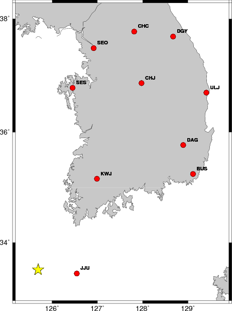
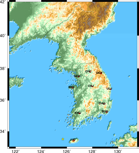
The focal mechanism was determined using broadband seismic waveforms. The location of the event and the and stations used for the waveform inversion are shown in the next figure.
|
|
|
|
The program wvfgrd96 was used with good traces observed at short distance to determine the focal mechanism, depth and seismic moment. This technique requires a high quality signal and well determined velocity model for the Green functions. To the extent that these are the quality data, this type of mechanism should be preferred over the radiation pattern technique which requires the separate step of defining the pressure and tension quadrants and the correct strike.
The observed and predicted traces are filtered using the following gsac commands:
hp c 0.02 n 3
lp c 0.10 n 3
The results of this grid search from 0.5 to 19 km depth are as follow:
           DEPTH  STK   DIP  RAKE   MW    FIT
WVFGRD96    0.5   270    60   -35   3.84 0.5917
WVFGRD96    1.0    95    50   -20   3.84 0.5867
WVFGRD96    2.0   100    60   -10   3.82 0.6131
WVFGRD96    3.0   100    65    -5   3.83 0.6451
WVFGRD96    4.0   100    65    -5   3.84 0.6701
WVFGRD96    5.0   100    70    -5   3.85 0.6890
WVFGRD96    6.0   100    70    -5   3.86 0.7062
WVFGRD96    7.0   100    70    -5   3.87 0.7204
WVFGRD96    8.0   100    70    -5   3.88 0.7320
WVFGRD96    9.0   100    70    -5   3.89 0.7410
WVFGRD96   10.0   100    70    -5   3.90 0.7470
WVFGRD96   11.0   100    70    -5   3.91 0.7507
WVFGRD96   12.0   105    70     0   3.92 0.7523
WVFGRD96   13.0   105    70     0   3.93 0.7525
WVFGRD96   14.0   105    70     5   3.94 0.7507
WVFGRD96   15.0   105    70     5   3.95 0.7474
WVFGRD96   16.0   105    70     5   3.95 0.7423
WVFGRD96   17.0   110    70     5   3.97 0.7352
WVFGRD96   18.0   110    70     5   3.98 0.7279
WVFGRD96   19.0   110    70     5   3.99 0.7198
WVFGRD96   20.0   110    70     5   3.99 0.7105
WVFGRD96   21.0   110    70    10   4.00 0.7005
WVFGRD96   22.0   110    70    10   4.01 0.6895
WVFGRD96   23.0   110    70    10   4.02 0.6778
WVFGRD96   24.0   110    75     5   4.02 0.6664
WVFGRD96   25.0   110    75     5   4.03 0.6570
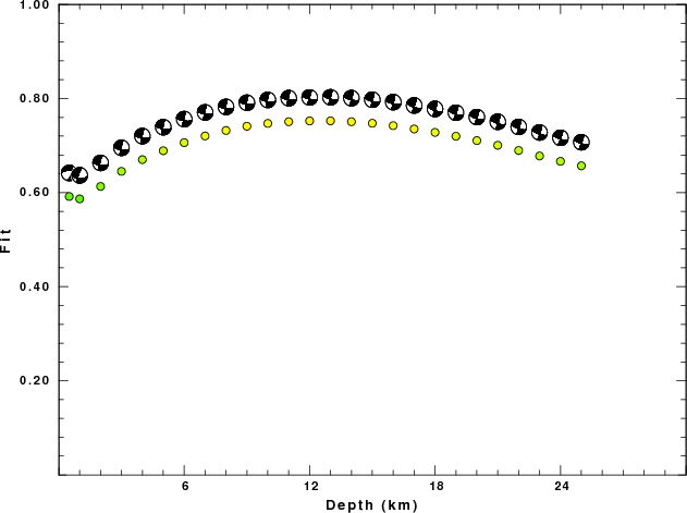
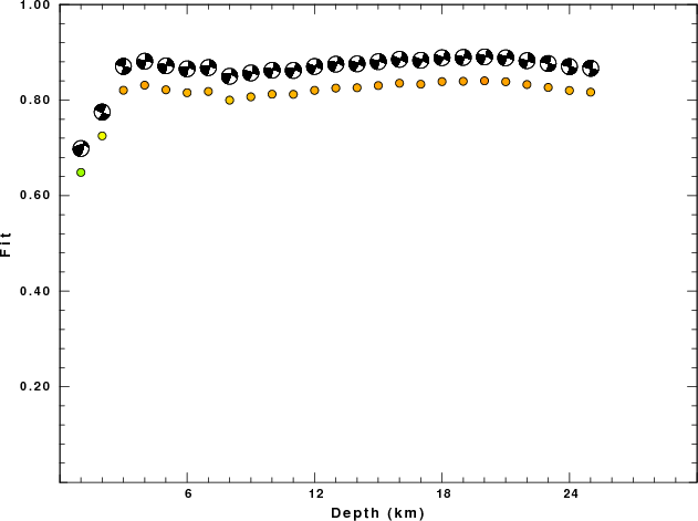
The best solution is
WVFGRD96 13.0 105 70 0 3.93 0.7525
The mechanism correspond to the best fit is
|
|
|
The best fit as a function of depth is given in the following figure:
|
|
|
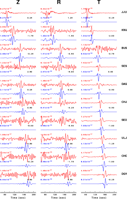
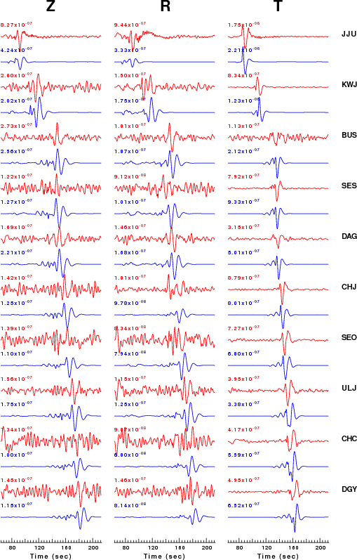
The comparison of the observed and predicted waveforms is given in the next figure. The red traces are the observed and the blue are the predicted. Each observed-predicted componnet is plotted to the same scale and peak amplitudes are indicated by the numbers to the left of each trace. The number in black at the rightr of each predicted traces it the time shift required for maximum correlation between the observed and predicted traces. This time shift is required because the synthetics are not computed at exactly the same distance as the observed and because the velocity model used in the predictions may not be perfect. A positive time shift indicates that the prediction is too fast and should be delayed to match the observed trace (shift to the right in this figure). A negative value indicates that the prediction is too slow. The bandpass filter used in the processing and for the display was
hp c 0.02 n 3
lp c 0.10 n 3
|
|
|
|
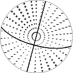
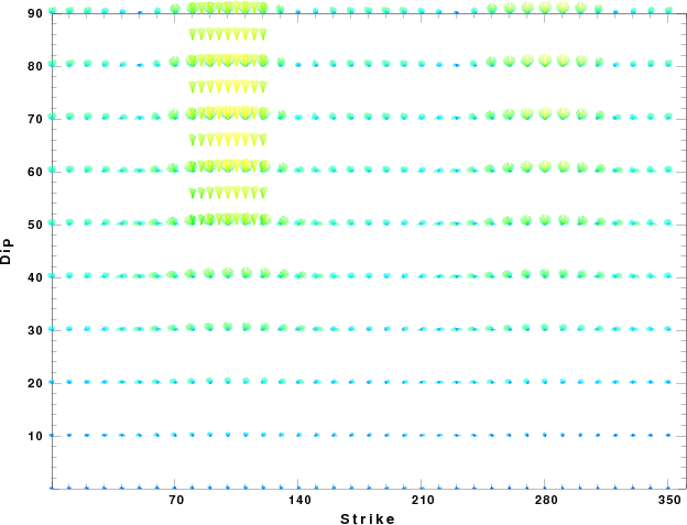
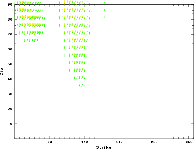
| Focal mechanism sensitivity at the preferred depth. The red color indicates a very good fit to thewavefroms. Each solution is plotted as a vector at a given value of strike and dip with the angle of the vector representing the rake angle, measured, with respect to the upward vertical (N) in the figure. |
The following figure shows the stations used in the grid search for the best focal mechanism to fit the surface-wave spectral amplitudes of the Love and Rayleigh waves.
|
|
|
The surface-wave determined focal mechanism is shown here.
  NODAL PLANES


  STK=     199.99
  DIP=      80.00
 RAKE=    -165.00

             OR

  STK=     107.32
  DIP=      75.23
 RAKE=     -10.35


DEPTH = 20.0 km

Mw = 4.01
Best Fit 0.8402 - P-T axis plot gives solutions with FIT greater than FIT90
 |
The P-wave first motion data for focal mechanism studies are as follow:
Sta Az    Dist   First motion
JJU        95   80 iP_D
KWJ        33  220 eP_X
BUS        57  370 eP_X
SES        11  371 eP_X
DAG        49  387 iP_D
CHJ        28  428 eP_X
SEO        14  456 eP_X
ULJ        43  491 eP_X
CHC        21  512 eP_X
DGY        29  538 eP_+
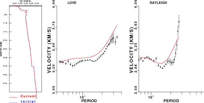
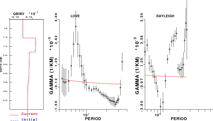
Surface wave analysis was performed using codes from Computer Programs in Seismology, specifically the multiple filter analysis program do_mft and the surface-wave radiation pattern search program srfgrd96.
Digital data were collected, instrument response removed and traces converted
to Z, R an T components. Multiple filter analysis was applied to the Z and T traces to obtain the Rayleigh- and Love-wave spectral amplitudes, respectively.
These were input to the search program which examined all depths between 1 and 25 km
and all possible mechanisms.
|
|
|
|
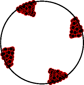
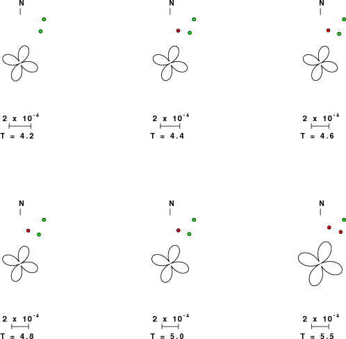
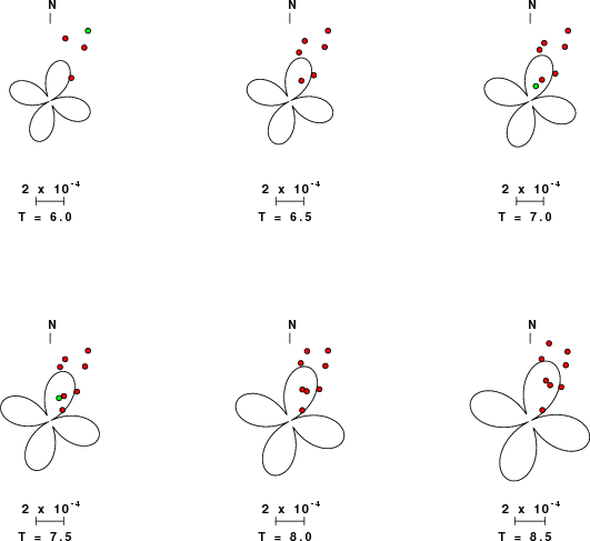
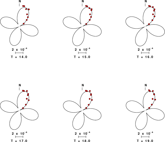
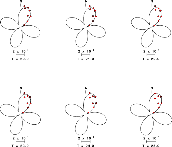
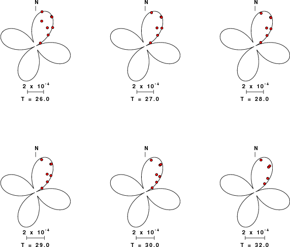
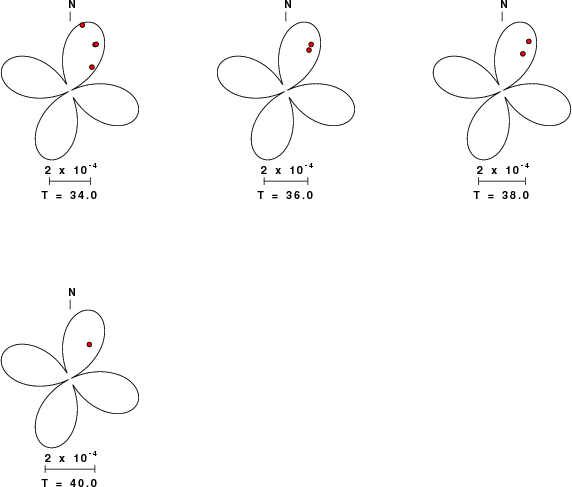
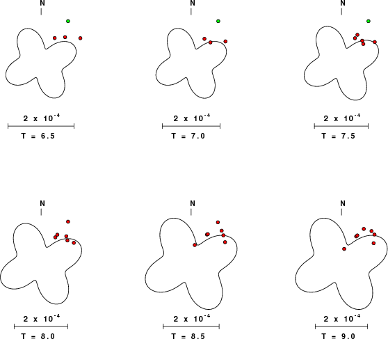
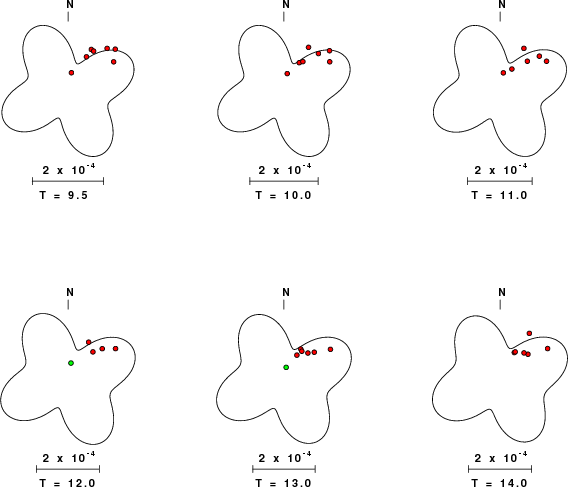
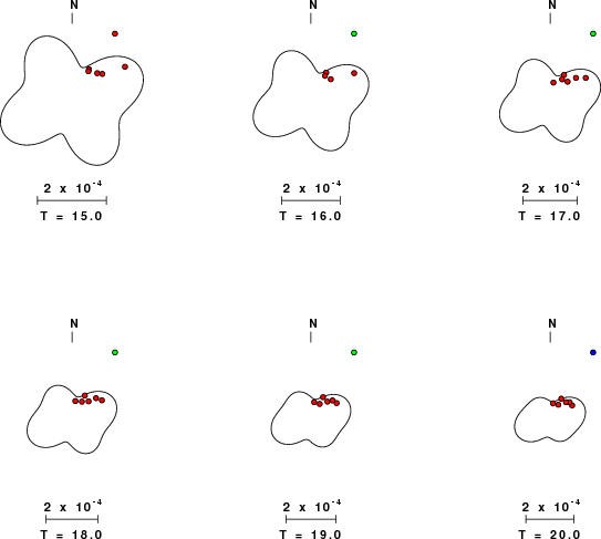
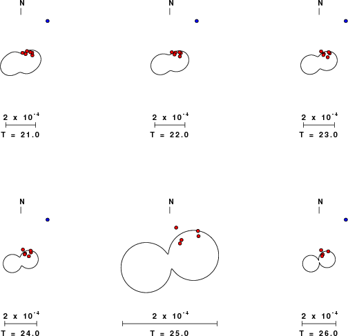
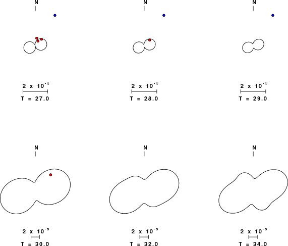
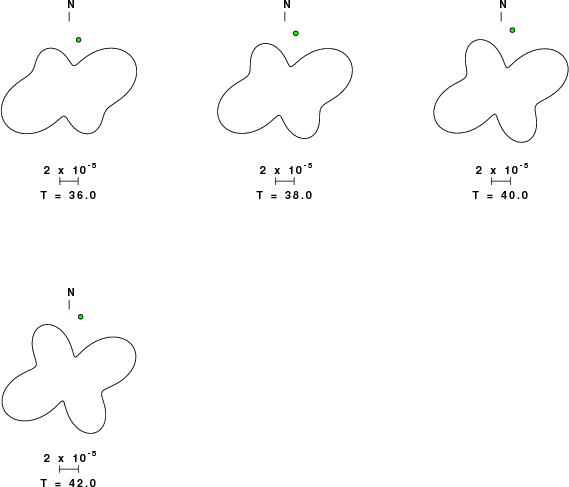
| Pressure-tension axis trends. Since the surface-wave spectra search does not distinguish between P and T axes and since there is a 180 ambiguity in strike, all possible P and T axes are plotted. First motion data and waveforms will be used to select the preferred mechanism. The purpose of this plot is to provide an idea of the possible range of solutions. The P and T-axes for all mechanisms with goodness of fit greater than 0.9 FITMAX (above) are plotted here. |
|
| Focal mechanism sensitivity at the preferred depth. The red color indicates a very good fit to the Love and Rayleigh wave radiation patterns. Each solution is plotted as a vector at a given value of strike and dip with the angle of the vector representing the rake angle, measured, with respect to the upward vertical (N) in the figure. Because of the symmetry of the spectral amplitude rediation patterns, only strikes from 0-180 degrees are sampled. |
The distribution of broadband stations with azimuth and distance is
Listing of broadband stations used
Since the analysis of the surface-wave radiation patterns uses only spectral amplitudes and because the surfave-wave radiation patterns have a 180 degree symmetry, each surface-wave solution consists of four possible focal mechanisms corresponding to the interchange of the P- and T-axes and a roation of the mechanism by 180 degrees. To select one mechanism, P-wave first motion can be used. This was not possible in this case because all the P-wave first motions were emergent ( a feature of the P-wave wave takeoff angle, the station location and the mechanism). The other way to select among the mechanisms is to compute forward synthetics and compare the observed and predicted waveforms.
The fits to the waveforms with the given mechanism are show below:
|
This figure shows the fit to the three components of motion (Z - vertical, R-radial and T - transverse). For each station and component, the observed traces is shown in red and the model predicted trace in blue. The traces represent filtered ground velocity in units of meters/sec (the peak value is printed adjacent to each trace; each pair of traces to plotted to the same scale to emphasize the difference in levels). Both synthetic and observed traces have been filtered using the SAC commands:
hp c 0.02 n 3
lp c 0.10 n 3
|
|
The digital data are provided by the Korea Meteorological Administration.
The t6.invSNU.CUVEL used for the waveform synthetic seismograms and for the surface wave eigenfunctions and dispersion is as follows:
MODEL.01
Model after    30 iterations
ISOTROPIC
KGS
SPHERICAL EARTH
1-D
CONSTANT VELOCITY
LINE08
LINE09
LINE10
LINE11
      H(KM)   VP(KM/S)   VS(KM/S) RHO(GM/CC)         QP         QS       ETAP       ETAS      FREFP      FREFS
     1.0000     5.3800     3.0009     2.5772  0.118E-02  0.167E-02   0.00       0.00       1.00       1.00
     1.0000     5.8057     3.2383     2.6606  0.118E-02  0.167E-02   0.00       0.00       1.00       1.00
     1.0000     6.1732     3.4433     2.7513  0.118E-02  0.167E-02   0.00       0.00       1.00       1.00
     3.0000     6.2872     3.5067     2.7862  0.118E-02  0.167E-02   0.00       0.00       1.00       1.00
     5.0000     6.3245     3.5281     2.7970  0.118E-02  0.167E-02   0.00       0.00       1.00       1.00
     5.0000     6.4165     3.5788     2.8248  0.118E-02  0.167E-02   0.00       0.00       1.00       1.00
     4.0000     6.5576     3.6576     2.8653  0.118E-02  0.167E-02   0.00       0.00       1.00       1.00
     5.0000     6.6402     3.7038     2.8865  0.118E-02  0.167E-02   0.00       0.00       1.00       1.00
     2.5000     6.6540     3.7115     2.8897  0.118E-02  0.167E-02   0.00       0.00       1.00       1.00
     2.5000     7.0960     3.9579     3.0111  0.118E-02  0.167E-02   0.00       0.00       1.00       1.00
     2.5000     7.9155     4.4148     3.2804  0.118E-02  0.167E-02   0.00       0.00       1.00       1.00
     2.5000     7.8925     4.4019     3.2735  0.118E-02  0.167E-02   0.00       0.00       1.00       1.00
     5.0000     7.8665     4.3876     3.2643  0.118E-02  0.167E-02   0.00       0.00       1.00       1.00
     5.0000     7.5675     4.2211     3.1625  0.118E-02  0.167E-02   0.00       0.00       1.00       1.00
     5.0000     7.7550     4.3252     3.2262  0.118E-02  0.167E-02   0.00       0.00       1.00       1.00
     5.0000     7.7602     4.3280     3.2282  0.118E-02  0.167E-02   0.00       0.00       1.00       1.00
     5.0000     7.7958     4.3487     3.2398  0.118E-02  0.167E-02   0.00       0.00       1.00       1.00
     5.0000     7.7415     4.3195     3.2217  0.118E-02  0.167E-02   0.00       0.00       1.00       1.00
     5.0000     7.6497     4.2688     3.1915  0.118E-02  0.167E-02   0.00       0.00       1.00       1.00
     5.0000     7.6408     4.2653     3.1889  0.118E-02  0.167E-02   0.00       0.00       1.00       1.00
     5.0000     7.6666     4.2716     3.1976  0.118E-02  0.167E-02   0.00       0.00       1.00       1.00
     5.0000     7.6699     4.2830     3.1986  0.118E-02  0.167E-02   0.00       0.00       1.00       1.00
     5.0000     7.6780     4.2885     3.2014  0.118E-02  0.167E-02   0.00       0.00       1.00       1.00
     5.0000     7.6816     4.2896     3.2028  0.118E-02  0.167E-02   0.00       0.00       1.00       1.00
     5.0000     7.6946     4.2996     3.2072  0.118E-02  0.167E-02   0.00       0.00       1.00       1.00
    10.0000     7.7349     4.3197     3.2208  0.118E-02  0.167E-02   0.00       0.00       1.00       1.00
    10.0000     7.7791     4.3484     3.2355  0.118E-02  0.167E-02   0.00       0.00       1.00       1.00
    10.0000     7.8331     4.3722     3.2536  0.862E-02  0.131E-01   0.00       0.00       1.00       1.00
    10.0000     7.8824     4.3863     3.2703  0.862E-02  0.131E-01   0.00       0.00       1.00       1.00
    10.0000     7.9360     4.4024     3.2883  0.855E-02  0.131E-01   0.00       0.00       1.00       1.00
    10.0000     7.9967     4.4237     3.3088  0.847E-02  0.131E-01   0.00       0.00       1.00       1.00
    10.0000     8.0529     4.4423     3.3289  0.847E-02  0.131E-01   0.00       0.00       1.00       1.00
    10.0000     8.1110     4.4603     3.3496  0.833E-02  0.130E-01   0.00       0.00       1.00       1.00
    10.0000     8.1762     4.4832     3.3728  0.826E-02  0.129E-01   0.00       0.00       1.00       1.00
    10.0000     8.2410     4.5054     3.3959  0.813E-02  0.128E-01   0.00       0.00       1.00       1.00
    10.0000     8.3022     4.5257     3.4176  0.806E-02  0.126E-01   0.00       0.00       1.00       1.00
    10.0000     8.3635     4.5514     3.4395  0.474E-02  0.746E-02   0.00       0.00       1.00       1.00
    10.0000     8.4257     4.5839     3.4617  0.472E-02  0.741E-02   0.00       0.00       1.00       1.00
    10.0000     8.4845     4.6145     3.4827  0.469E-02  0.741E-02   0.00       0.00       1.00       1.00
    10.0000     8.5403     4.6434     3.5020  0.467E-02  0.735E-02   0.00       0.00       1.00       1.00
    10.0000     8.5934     4.6708     3.5199  0.465E-02  0.735E-02   0.00       0.00       1.00       1.00
    10.0000     8.6436     4.6959     3.5369  0.463E-02  0.730E-02   0.00       0.00       1.00       1.00
    10.0000     8.6912     4.7194     3.5530  0.461E-02  0.730E-02   0.00       0.00       1.00       1.00
    10.0000     8.7365     4.7413     3.5684  0.459E-02  0.725E-02   0.00       0.00       1.00       1.00
    10.0000     8.7797     4.7622     3.5831  0.455E-02  0.725E-02   0.00       0.00       1.00       1.00
    10.0000     8.8199     4.7819     3.5967  0.452E-02  0.719E-02   0.00       0.00       1.00       1.00
    10.0000     8.8587     4.8001     3.6099  0.450E-02  0.714E-02   0.00       0.00       1.00       1.00
    10.0000     8.8958     4.8177     3.6226  0.448E-02  0.714E-02   0.00       0.00       1.00       1.00
    10.0000     8.9314     4.8346     3.6347  0.446E-02  0.709E-02   0.00       0.00       1.00       1.00
    10.0000     8.9647     4.8500     3.6461  0.442E-02  0.704E-02   0.00       0.00       1.00       1.00
    10.0000     8.9962     4.8651     3.6569  0.441E-02  0.704E-02   0.00       0.00       1.00       1.00
    10.0000     9.0263     4.8783     3.6685  0.439E-02  0.699E-02   0.00       0.00       1.00       1.00
    10.0000     9.0547     4.8915     3.6800  0.435E-02  0.694E-02   0.00       0.00       1.00       1.00
    10.0000     9.0822     4.9041     3.6911  0.433E-02  0.690E-02   0.00       0.00       1.00       1.00
    10.0000     9.1091     4.9164     3.7020  0.431E-02  0.690E-02   0.00       0.00       1.00       1.00
    10.0000     9.1346     4.9280     3.7123  0.427E-02  0.685E-02   0.00       0.00       1.00       1.00
    10.0000     9.4876     5.1513     3.8537  0.388E-02  0.613E-02   0.00       0.00       1.00       1.00
    10.0000     9.5095     5.1663     3.8624  0.388E-02  0.613E-02   0.00       0.00       1.00       1.00
    10.0000     9.5299     5.1806     3.8703  0.386E-02  0.610E-02   0.00       0.00       1.00       1.00
    10.0000     9.5507     5.1944     3.8784  0.386E-02  0.610E-02   0.00       0.00       1.00       1.00
    10.0000     9.5706     5.2080     3.8861  0.385E-02  0.606E-02   0.00       0.00       1.00       1.00
    10.0000     9.5900     5.2214     3.8937  0.385E-02  0.606E-02   0.00       0.00       1.00       1.00
    10.0000     9.6090     5.2347     3.9011  0.383E-02  0.606E-02   0.00       0.00       1.00       1.00
    10.0000     9.6272     5.2480     3.9081  0.383E-02  0.602E-02   0.00       0.00       1.00       1.00
    10.0000     9.6458     5.2604     3.9154  0.383E-02  0.602E-02   0.00       0.00       1.00       1.00
    10.0000     9.6794     5.2816     3.9282  0.382E-02  0.599E-02   0.00       0.00       1.00       1.00
    10.0000     9.7130     5.3029     3.9409  0.382E-02  0.599E-02   0.00       0.00       1.00       1.00
    10.0000     9.7466     5.3242     3.9537  0.380E-02  0.599E-02   0.00       0.00       1.00       1.00
    10.0000     9.7799     5.3454     3.9664  0.380E-02  0.595E-02   0.00       0.00       1.00       1.00
    10.0000     9.8137     5.3669     3.9792  0.380E-02  0.595E-02   0.00       0.00       1.00       1.00
    10.0000     9.8473     5.3883     3.9920  0.379E-02  0.592E-02   0.00       0.00       1.00       1.00
    10.0000     9.8808     5.4094     4.0047  0.379E-02  0.592E-02   0.00       0.00       1.00       1.00
     0.0000     9.9144     5.4306     4.0175  0.377E-02  0.592E-02   0.00       0.00       1.00       1.00
Here we tabulate the reasons for not using certain digital data sets
The following stations did not have a valid response files:
DATE=Sat May 31 20:20:58 CDT 2008