2003/03/30 11:10:56 37.57N 123.82E 3 4.60 Korea
 SLU Moment Tensor Solution
 2003/03/30 11:10:56 37.57N 123.82E 3 4.60 Korea

 Best Fitting Double Couple
    Mo = 8.91e+22 dyne-cm
    Mw = 4.60
    Z  = 13 km
     Plane   Strike  Dip  Rake
      NP1      187    77   149
      NP2      285    60    15
 Principal Axes:
   Axis    Value   Plunge  Azimuth
     T   8.91e+22     31     142
     N   0.00e+00     57     347
     P  -8.91e+22     11     239


 Moment Tensor: (dyne-cm)
    Component  Value
       Mxx     1.86e+22
       Mxy    -6.96e+22
       Mxz    -2.23e+22
       Myy    -3.86e+22
       Myz     3.86e+22
       Mzz     2.00e+22


                     #########-----
                 ############----------
              ##############--------------
             ###############---------------
           ################------------------
          #################-------------------
         #######---------#---------------------
        ##----------------#######---------------
        -----------------############-----------
       ------------------###############---------
       ------------------##################------
       ------------------####################----
       -----------------######################---
        ----------------########################
        ----------------########################
         --   ----------#######################
          - P ----------###########   ########
              ----------########### T #######
             -----------###########   #####
              ----------##################
                 --------##############
                     ----##########


 Harvard Convention
 Moment Tensor:
      R          T          F
  2.00e+22  -2.23e+22  -3.86e+22
 -2.23e+22   1.86e+22   6.96e+22
 -3.86e+22   6.96e+22  -3.86e+22
|
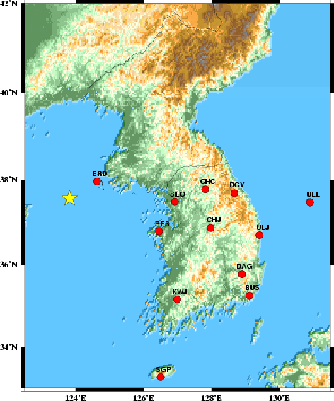
The focal mechanism was determined using broadband seismic waveforms. The location of the event and the station distribution are given in Figure 1.
|
|
|
|
      STK = 285
      DIP = 60
     RAKE = 15
       MW = 4.60
       HS = 13
The waveform inversion is preferred. This solution agrees with the surface-wave solution. This solution is well determined.
The program wvfgrd96 was used with good traces observed at short distance to determine the focal mechanism, depth and seismic moment. This technique requires a high quality signal and well determined velocity model for the Green functions. To the extent that these are the quality data, this type of mechanism should be preferred over the radiation pattern technique which requires the separate step of defining the pressure and tension quadrants and the correct strike.
The observed and predicted traces are filtered using the following gsac commands:
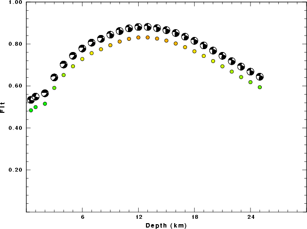
hp c 0.02 3
lp c 0.10 3
The results of this grid search from 0.5 to 19 km depth are as follow:
           DEPTH  STK   DIP  RAKE   MW    FIT
WVFGRD96    0.5   105    80   -25   4.39 0.4839
WVFGRD96    1.0   105    80   -10   4.39 0.4993
WVFGRD96    2.0   275    65   -50   4.54 0.5153
WVFGRD96    3.0   275    55   -40   4.54 0.5907
WVFGRD96    4.0   275    55   -40   4.55 0.6521
WVFGRD96    5.0   275    55   -40   4.55 0.6937
WVFGRD96    6.0   280    60   -30   4.54 0.7283
WVFGRD96    7.0   280    60   -30   4.55 0.7562
WVFGRD96    8.0   280    60   -30   4.55 0.7747
WVFGRD96    9.0   285    55    15   4.55 0.7940
WVFGRD96   10.0   285    55    15   4.56 0.8115
WVFGRD96   11.0   285    60    15   4.58 0.8243
WVFGRD96   12.0   285    60    15   4.59 0.8309
WVFGRD96   13.0   285    60    15   4.60 0.8311
WVFGRD96   14.0   285    60    15   4.60 0.8255
WVFGRD96   15.0   285    60    15   4.61 0.8159
WVFGRD96   16.0   285    60    15   4.62 0.8022
WVFGRD96   17.0   285    60    15   4.63 0.7847
WVFGRD96   18.0   285    55    15   4.63 0.7650
WVFGRD96   19.0   285    55    15   4.64 0.7430
WVFGRD96   20.0   285    60    15   4.66 0.7186
WVFGRD96   21.0   285    60    10   4.67 0.6936
WVFGRD96   22.0   285    60    10   4.67 0.6682
WVFGRD96   23.0   285    60    10   4.68 0.6423
WVFGRD96   24.0   285    60    10   4.69 0.6182
WVFGRD96   25.0   285    60     5   4.70 0.5940
The best solution is
WVFGRD96 13.0 285 60 15 4.60 0.8311
The mechanism correspond to the best fit is
|
|
|
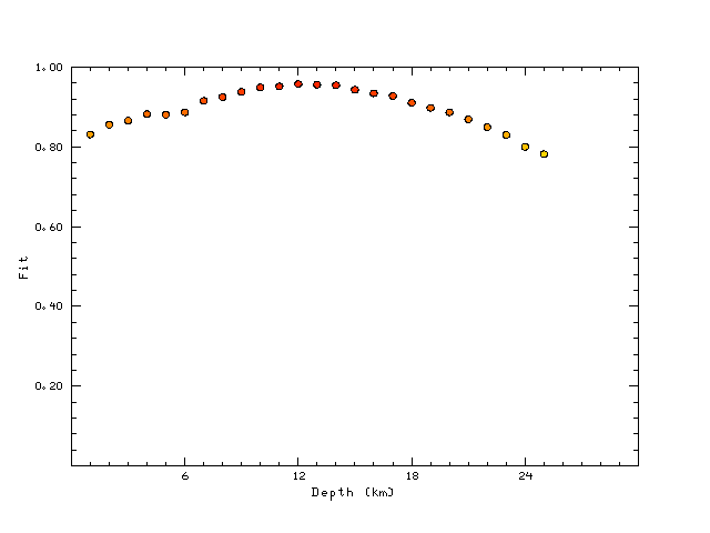
The best fit as a function of depth is given in the following figure:
|
|
|
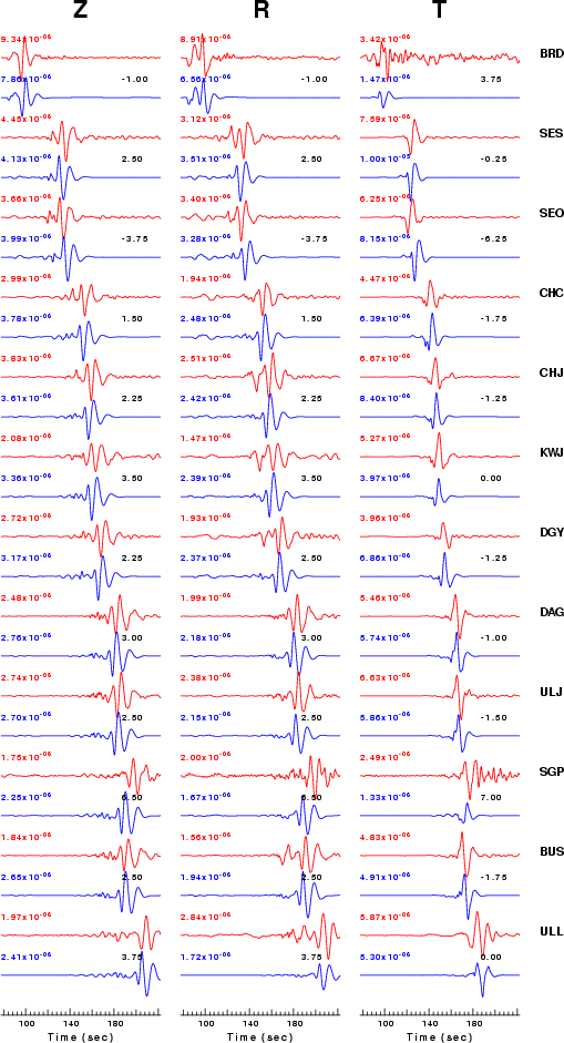
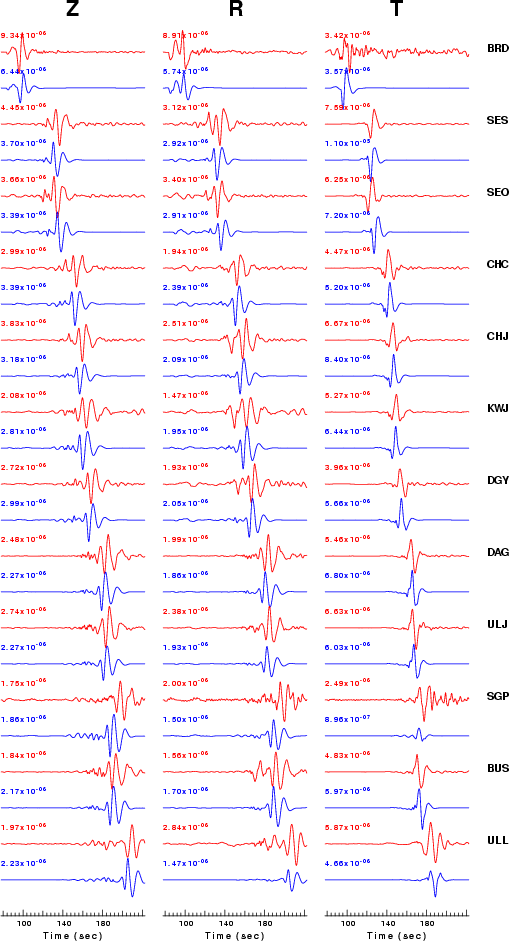
The comparison of the observed and predicted waveforms is given in the next figure. The red traces are the observed and the blue are the predicted. Each observed-predicted componnet is plotted to the same scale and peak amplitudes are indicated by the numbers to the left of each trace. The number in black at the rightr of each predicted traces it the time shift required for maximum correlation between the observed and predicted traces. This time shift is required because the synthetics are not computed at exactly the same distance as the observed and because the velocity model used in the predictions may not be perfect. A positive time shift indicates that the prediction is too fast and should be delayed to match the observed trace (shift to the right in this figure). A negative value indicates that the prediction is too slow. The bandpass filter used in the processing and for the display was
hp c 0.02 3
lp c 0.10 3
|
|
|
|
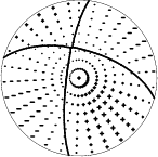
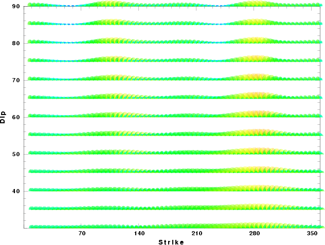
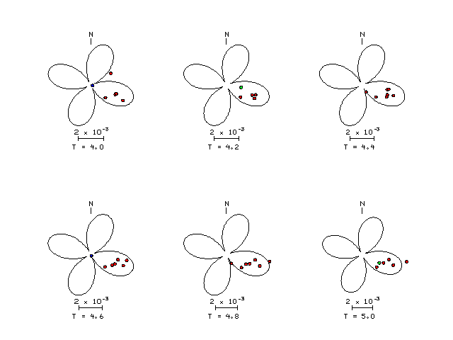
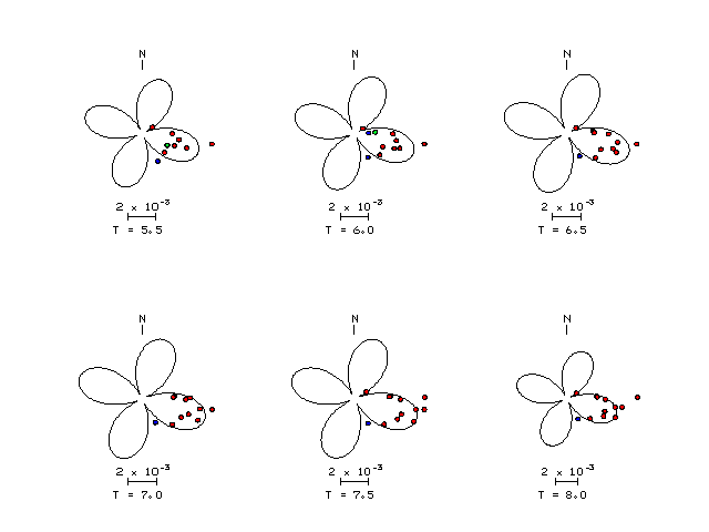
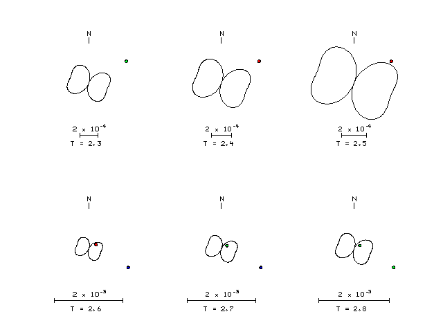
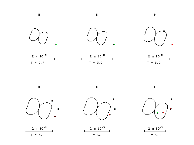
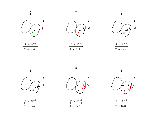
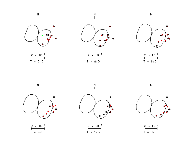
| Focal mechanism sensitivity at the preferred depth. The red color indicates a very good fit to thewavefroms. Each solution is plotted as a vector at a given value of strike and dip with the angle of the vector representing the rake angle, measured, with respect to the upward vertical (N) in the figure. |
  NODAL PLANES


  STK=      20.00
  DIP=      90.00
 RAKE=    -155.00

             OR

  STK=     290.00
  DIP=      65.00
 RAKE=      -0.01


DEPTH = 12.0 km

Mw = 4.58
Best Fit 0.95776 - P-T axis plot gives solutions with FIT greater than FIT90
 |
The P-wave first motion data for focal mechanism studies are as follow:
Sta Az(deg)    Dist(km)   First motion
BRD        58   84 iP_D
SES       110  249 iP_C
SEO        91  274 eP_+
CHC        85  353 eP_-
CHJ       101  377 eP_-
KWJ       132  390 eP_+
DGY        87  429 eP_-
DAG       112  496 eP_X
ULJ        99  506 eP_X
SGP       152  537 eP_X
BUS       117  540 eP_X
ULL        89  626 eP_X
Surface wave analysis was performed using codes from Computer Programs in Seismology, specifically the multiple filter analysis program do_mft and the surface-wave radiation pattern search program srfgrd96.
Digital data were collected, instrument response removed and traces converted
to Z, R an T components. Multiple filter analysis was applied to the Z and T traces to obtain the Rayleigh- and Love-wave spectral amplitudes, respectively.
These were input to the search program which examined all depths between 1 and 25 km
and all possible mechanisms.
|
|
|
|
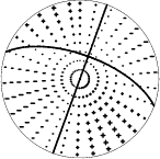
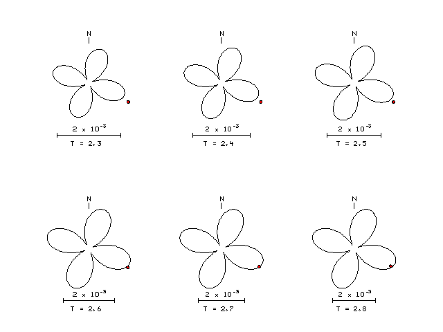
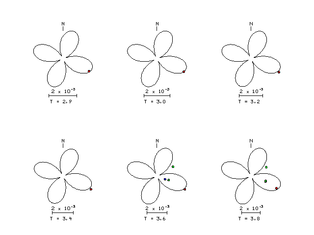
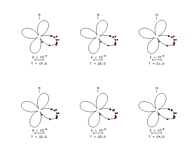
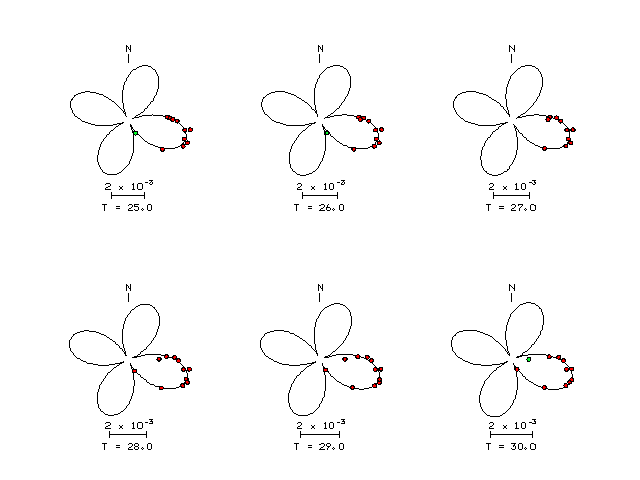
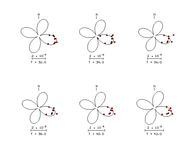
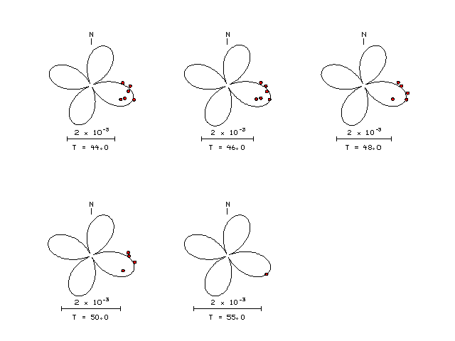
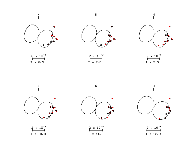
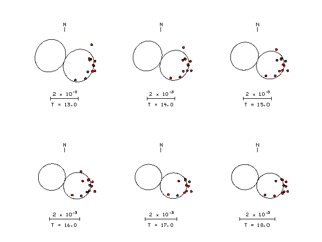
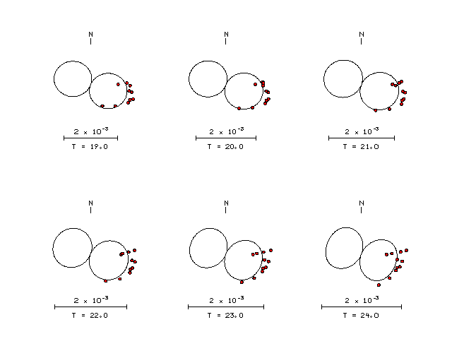
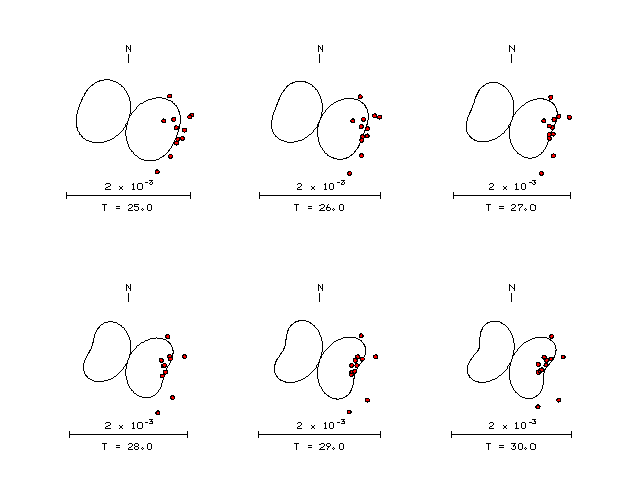
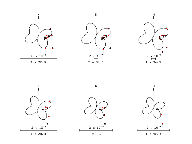
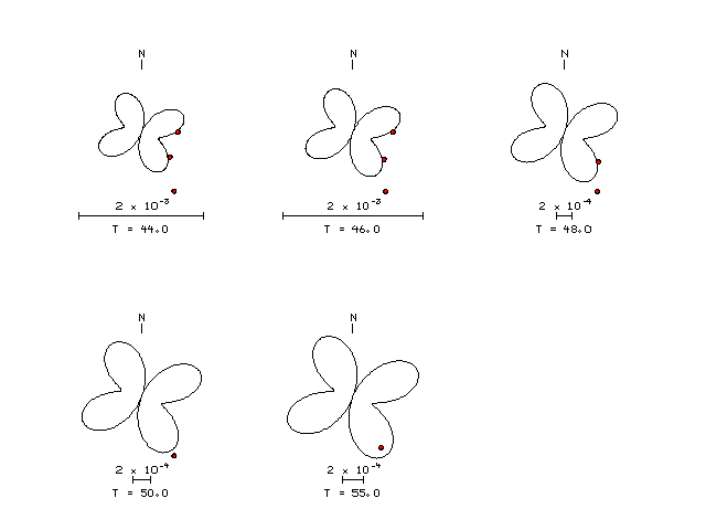
| Pressure-tension axis trends. Since the surface-wave spectra search does not distinguish between P and T axes and since there is a 180 ambiguity in strike, all possible P and T axes are plotted. First motion data and waveforms will be used to select the preferred mechanism. The purpose of this plot is to provide an idea of the possible range of solutions. The P and T-axes for all mechanisms with goodness of fit greater than 0.9 FITMAX (above) are plotted here. |
|
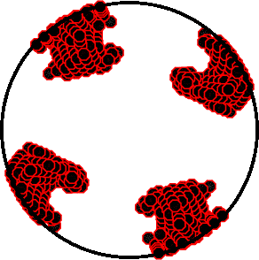
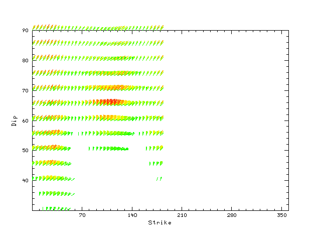
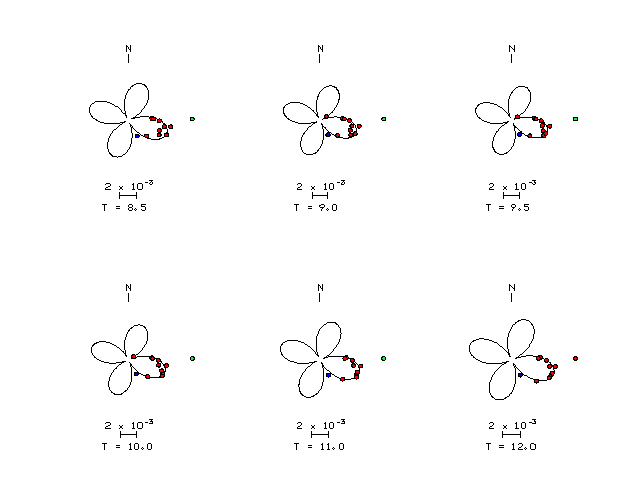
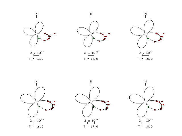
| Focal mechanism sensitivity at the preferred depth. The red color indicates a very good fit to the Love and Rayleigh wave radiation patterns. Each solution is plotted as a vector at a given value of strike and dip with the angle of the vector representing the rake angle, measured, with respect to the upward vertical (N) in the figure. Because of the symmetry of the spectral amplitude rediation patterns, only strikes from 0-180 degrees are sampled. |
The distribution of broadband stations with azimuth and distance is
Sta Az(deg)    Dist(km)
BRD	   58	   84
SES	  110	  249
SEO	   91	  274
CHC	   85	  353
CHJ	  101	  377
KWJ	  132	  390
DGY	   87	  429
DAG	  112	  496
ULJ	   99	  506
SGP	  152	  537
BUS	  117	  540
ULL	   89	  626
Since the analysis of the surface-wave radiation patterns uses only spectral amplitudes and because the surfave-wave radiation patterns have a 180 degree symmetry, each surface-wave solution consists of four possible focal mechanisms corresponding to the interchange of the P- and T-axes and a roation of the mechanism by 180 degrees. To select one mechanism, P-wave first motion can be used. This was not possible in this case because all the P-wave first motions were emergent ( a feature of the P-wave wave takeoff angle, the station location and the mechanism). The other way to select among the mechanisms is to compute forward synthetics and compare the observed and predicted waveforms.
The fits to the waveforms with the given mechanism are show below:
|
This figure shows the fit to the three components of motion (Z - vertical, R-radial and T - transverse). For each station and component, the observed traces is shown in red and the model predicted trace in blue. The traces represent filtered ground velocity in units of meters/sec (the peak value is printed adjacent to each trace; each pair of traces to plotted to the same scale to emphasize the difference in levels). Both synthetic and observed traces have been filtered using the SAC commands:
hp c 0.02 3
lp c 0.10 3
|
|
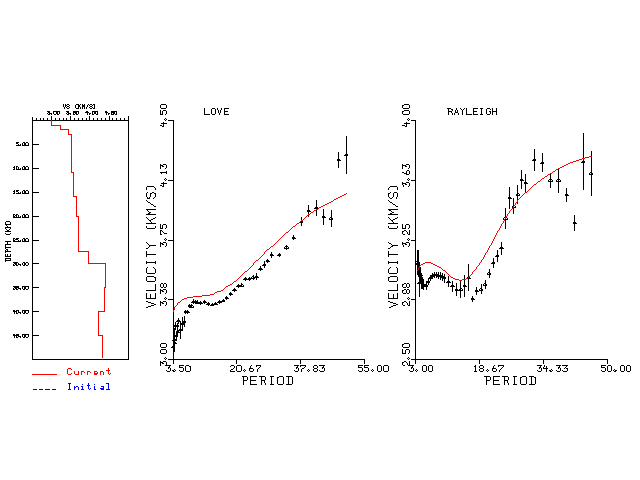
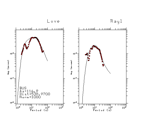
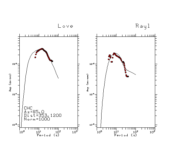
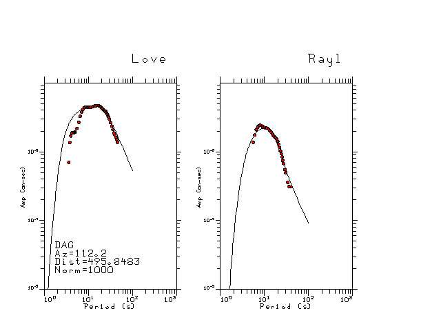
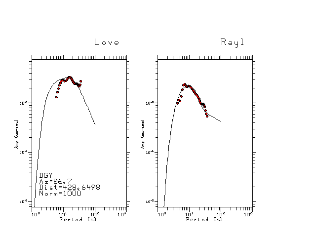
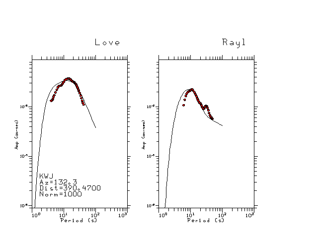
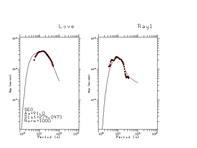
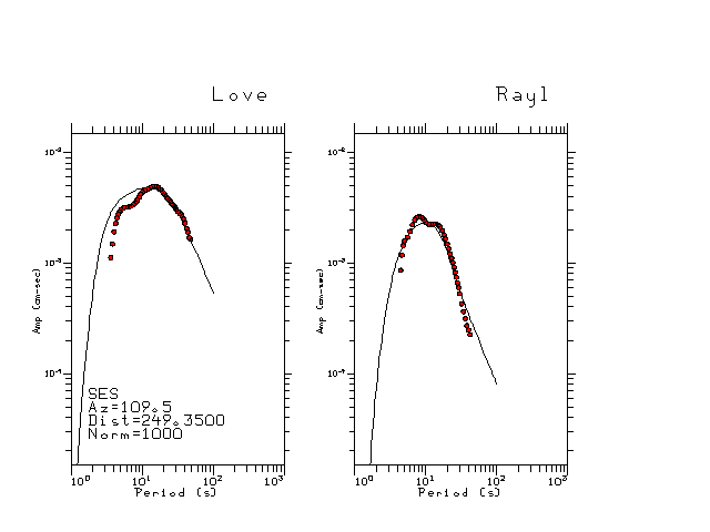
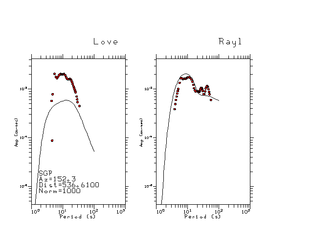
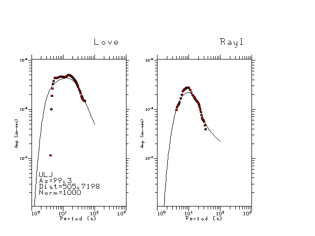
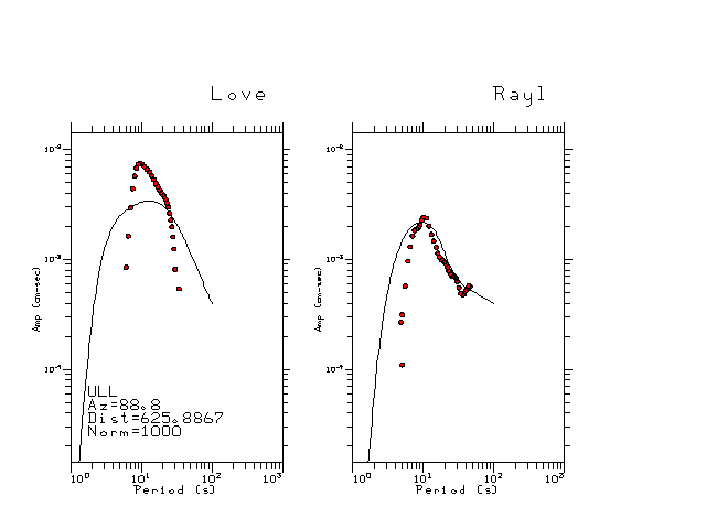
The figures below show the observed spectral amplitudes (units of cm-sec) at each station and the
theoretical predictions as a function of period for the mechanism given above. The modified Utah model earth model
was used to define the Green's functions. For each station, the Love and Rayleigh wave spectrail amplitudes are plotted with the same scaling so that one can get a sense fo the effects of the effects of the focal mechanism and depth on the excitation of each.
 |
 |
 |
 |
 |
 |
 |
 |
 |
 |
 |
 |
Here we tabulate the reasons for not using certain digital data sets