Location
2017/11/19 12:37:43 44.66 10.07 32.0 4.4 Fornovp
Arrival Times (from USGS)
Arrival time list
Felt Map
USGS Felt map for this earthquake
USGS Felt reports page for
Focal Mechanism
 SLU Moment Tensor Solution
 ENS  2017/11/19 12:37:43:0  44.66   10.07  32.0 4.4 Fornovp

 Stations used:
   CH.BERNI CH.MUGIO FR.ESCA FR.MON FR.SAOF FR.SPIF FR.TURF
   GU.RSP IV.BRMO IV.CASP IV.CELB IV.CRMI IV.CSNT IV.IMI
   IV.MSSA IV.OSSC IV.PARC IV.PLMA IV.QLNO IV.SALO MN.VLC

 Filtering commands used:
   cut o DIST/3.3 -20 o DIST/3.3 +50
   rtr
   taper w 0.1
   hp c 0.03 n 3
   lp c 0.10 n 3

 Best Fitting Double Couple
  Mo = 3.31e+22 dyne-cm
  Mw = 4.28
  Z  = 20 km
  Plane   Strike  Dip  Rake
   NP1      337    58   116
   NP2      115    40    55
  Principal Axes:
   Axis    Value   Plunge  Azimuth
    T   3.31e+22     66     297
    N   0.00e+00     22     143
    P  -3.31e+22     10      49

 Moment Tensor: (dyne-cm)
    Component   Value
       Mxx    -1.26e+22
       Mxy    -1.81e+22
       Mxz     1.88e+21
       Myy    -1.41e+22
       Myz    -1.52e+22
       Mzz     2.67e+22


                     --------------
                 #######---------------
              ############----------------
             ###############-------------
           ###################----------- P -
          ######################---------   --
         ########################--------------
        -#########################--------------
        --###########   ###########-------------
       ---########### T ############-------------
       ----##########   ############-------------
       -----#########################------------
       ------########################------------
        ------########################----------
        --------######################----------
         ---------####################---------
          -----------#################-------#
           --------------#############----###
             -------------------------#####
              -----------------------#####
                 --------------------##
                     --------------


 Global CMT Convention Moment Tensor:
      R          T          P
  2.67e+22   1.88e+21   1.52e+22
  1.88e+21  -1.26e+22   1.81e+22
  1.52e+22   1.81e+22  -1.41e+22


Details of the solution is found at

http://www.eas.slu.edu/eqc/eqc_mt/MECH.IT/20171119123743/index.html
|
Preferred Solution
The preferred solution from an analysis of the surface-wave spectral amplitude radiation pattern, waveform inversion and first motion observations is
      STK = 115
      DIP = 40
     RAKE = 55
       MW = 4.28
       HS = 20.0
The NDK file is 20171119123743.ndk
The waveform inversion is preferred.
Moment Tensor Comparison
The following compares this source inversion to others
| SLU |
INGVTDMT |
 SLU Moment Tensor Solution
 ENS  2017/11/19 12:37:43:0  44.66   10.07  32.0 4.4 Fornovp

 Stations used:
   CH.BERNI CH.MUGIO FR.ESCA FR.MON FR.SAOF FR.SPIF FR.TURF
   GU.RSP IV.BRMO IV.CASP IV.CELB IV.CRMI IV.CSNT IV.IMI
   IV.MSSA IV.OSSC IV.PARC IV.PLMA IV.QLNO IV.SALO MN.VLC

 Filtering commands used:
   cut o DIST/3.3 -20 o DIST/3.3 +50
   rtr
   taper w 0.1
   hp c 0.03 n 3
   lp c 0.10 n 3

 Best Fitting Double Couple
  Mo = 3.31e+22 dyne-cm
  Mw = 4.28
  Z  = 20 km
  Plane   Strike  Dip  Rake
   NP1      337    58   116
   NP2      115    40    55
  Principal Axes:
   Axis    Value   Plunge  Azimuth
    T   3.31e+22     66     297
    N   0.00e+00     22     143
    P  -3.31e+22     10      49

 Moment Tensor: (dyne-cm)
    Component   Value
       Mxx    -1.26e+22
       Mxy    -1.81e+22
       Mxz     1.88e+21
       Myy    -1.41e+22
       Myz    -1.52e+22
       Mzz     2.67e+22


                     --------------
                 #######---------------
              ############----------------
             ###############-------------
           ###################----------- P -
          ######################---------   --
         ########################--------------
        -#########################--------------
        --###########   ###########-------------
       ---########### T ############-------------
       ----##########   ############-------------
       -----#########################------------
       ------########################------------
        ------########################----------
        --------######################----------
         ---------####################---------
          -----------#################-------#
           --------------#############----###
             -------------------------#####
              -----------------------#####
                 --------------------##
                     --------------


 Global CMT Convention Moment Tensor:
      R          T          P
  2.67e+22   1.88e+21   1.52e+22
  1.88e+21  -1.26e+22   1.81e+22
  1.52e+22   1.81e+22  -1.41e+22


Details of the solution is found at

http://www.eas.slu.edu/eqc/eqc_mt/MECH.IT/20171119123743/index.html
|
|
Magnitudes
ML Magnitude
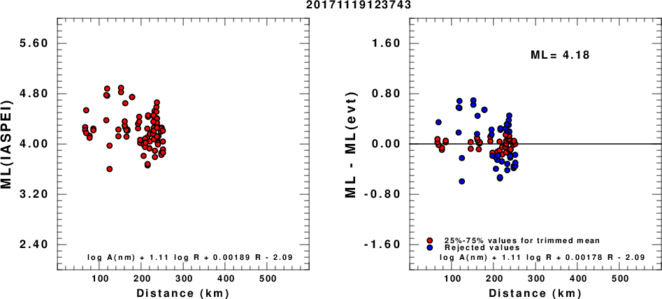
(a) ML computed using the IASPEI formula for Horizontal components; (b) ML residuals computed using a modified IASPEI formula that accounts for path specific attenuation; the values used for the trimmed mean are indicated. The ML relation used for each figure is given at the bottom of each plot.
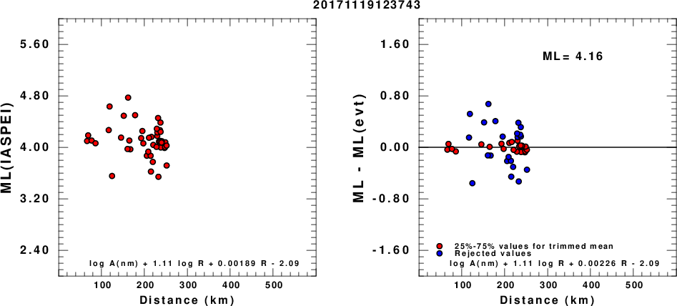
(a) ML computed using the IASPEI formula for Vertical components (research); (b) ML residuals computed using a modified IASPEI formula that accounts for path specific attenuation; the values used for the trimmed mean are indicated. The ML relation used for each figure is given at the bottom of each plot.
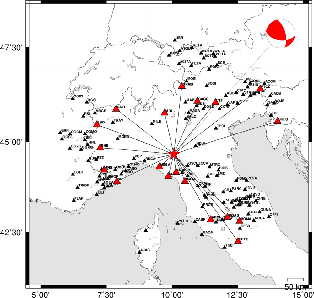
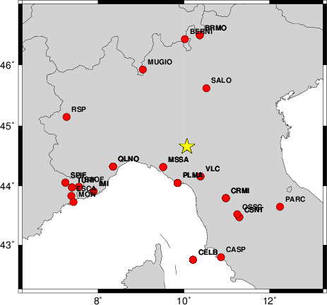
Waveform Inversion
The focal mechanism was determined using broadband seismic waveforms. The location of the event and the
and stations used for the waveform inversion are shown in the next figure.
|
|
Location of broadband stations used for waveform inversion
|
The program wvfgrd96 was used with good traces observed at short distance to determine the focal mechanism, depth and seismic moment. This technique requires a high quality signal and well determined velocity model for the Green functions. To the extent that these are the quality data, this type of mechanism should be preferred over the radiation pattern technique which requires the separate step of defining the pressure and tension quadrants and the correct strike.
The observed and predicted traces are filtered using the following gsac commands:
cut o DIST/3.3 -20 o DIST/3.3 +50
rtr
taper w 0.1
hp c 0.03 n 3
lp c 0.10 n 3
The results of this grid search from 0.5 to 19 km depth are as follow:
           DEPTH  STK   DIP  RAKE   MW    FIT
WVFGRD96    1.0   320    45   -90   3.92 0.3696
WVFGRD96    2.0   140    40   -90   3.99 0.3595
WVFGRD96    3.0   300    45    60   3.96 0.2700
WVFGRD96    4.0    90    60   -30   3.93 0.2819
WVFGRD96    5.0    80    45   -30   4.02 0.2965
WVFGRD96    6.0    80    35   -10   4.03 0.3286
WVFGRD96    7.0    90    30    10   4.06 0.3661
WVFGRD96    8.0    85    35     5   4.04 0.4032
WVFGRD96    9.0    95    35    20   4.07 0.4368
WVFGRD96   10.0    95    35    20   4.09 0.4681
WVFGRD96   11.0   100    40    30   4.11 0.4981
WVFGRD96   12.0   105    40    35   4.13 0.5257
WVFGRD96   13.0   105    45    40   4.15 0.5517
WVFGRD96   14.0   110    45    50   4.17 0.5780
WVFGRD96   15.0   115    45    55   4.21 0.6056
WVFGRD96   16.0   115    45    55   4.23 0.6300
WVFGRD96   17.0   115    40    55   4.24 0.6490
WVFGRD96   18.0   115    40    55   4.25 0.6645
WVFGRD96   19.0   115    40    55   4.27 0.6743
WVFGRD96   20.0   115    40    55   4.28 0.6784
WVFGRD96   21.0   115    40    55   4.29 0.6779
WVFGRD96   22.0   115    35    50   4.30 0.6744
WVFGRD96   23.0   115    35    50   4.31 0.6672
WVFGRD96   24.0   115    35    50   4.31 0.6545
WVFGRD96   25.0   110    35    45   4.32 0.6380
WVFGRD96   26.0   110    35    40   4.33 0.6201
WVFGRD96   27.0   110    35    40   4.34 0.6028
WVFGRD96   28.0   110    30    40   4.34 0.5883
WVFGRD96   29.0   110    30    40   4.35 0.5764
The best solution is
WVFGRD96 20.0 115 40 55 4.28 0.6784
The mechanism correspond to the best fit is
|
|
Figure 1. Waveform inversion focal mechanism
|
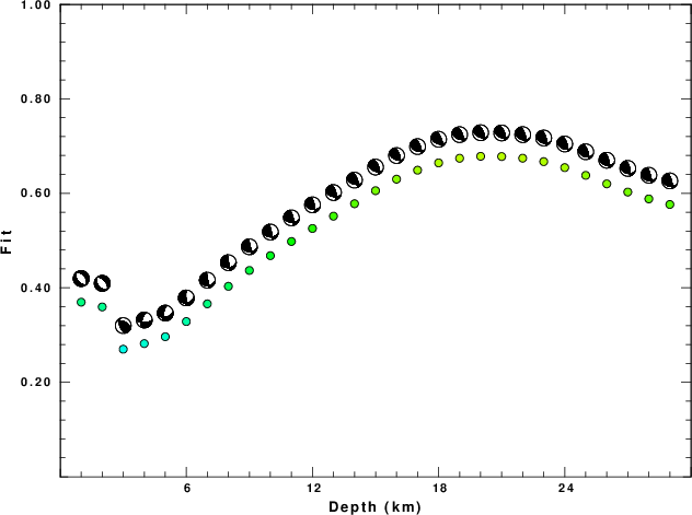
The best fit as a function of depth is given in the following figure:
|
|
Figure 2. Depth sensitivity for waveform mechanism
|
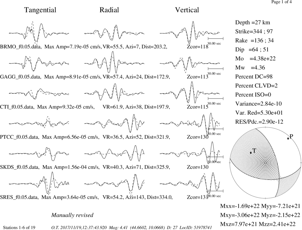
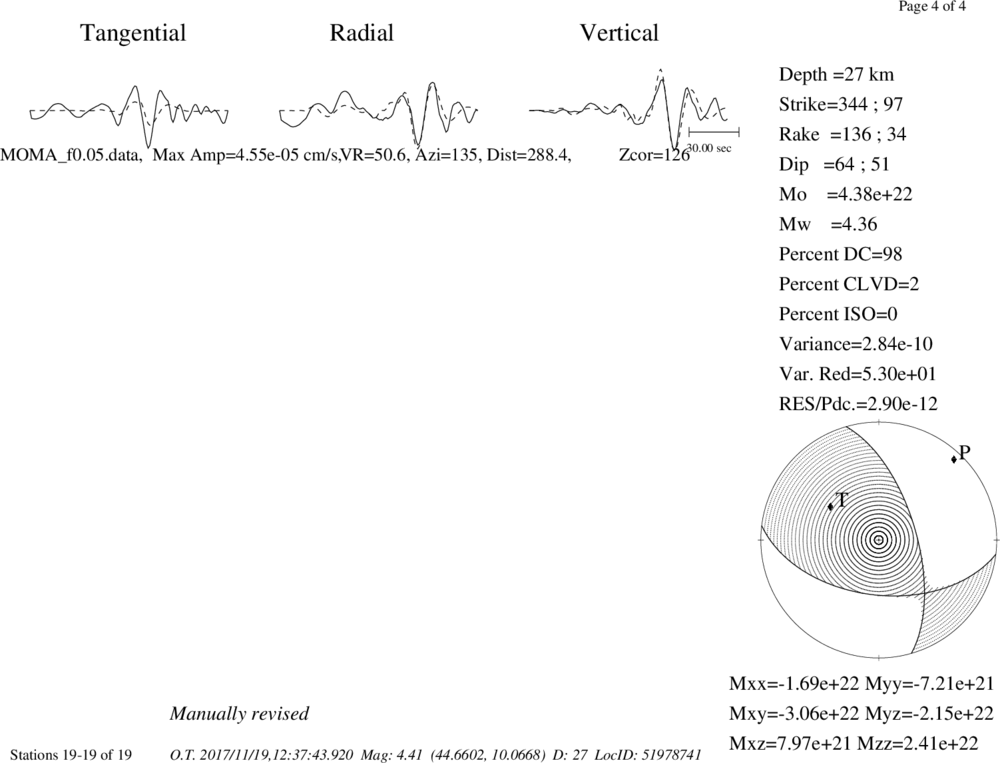
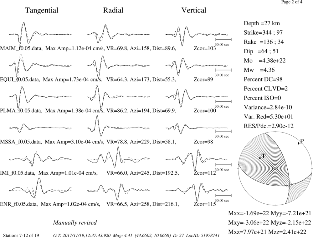
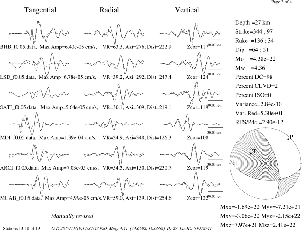
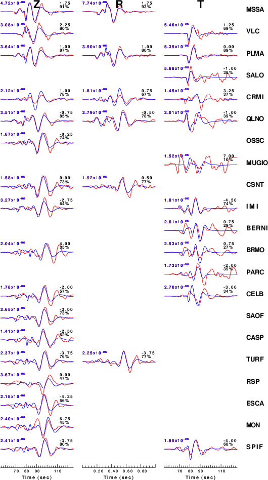
The comparison of the observed and predicted waveforms is given in the next figure. The red traces are the observed and the blue are the predicted.
Each observed-predicted component is plotted to the same scale and peak amplitudes are indicated by the numbers to the left of each trace. A pair of numbers is given in black at the right of each predicted traces. The upper number it the time shift required for maximum correlation between the observed and predicted traces. This time shift is required because the synthetics are not computed at exactly the same distance as the observed and because the velocity model used in the predictions may not be perfect.
A positive time shift indicates that the prediction is too fast and should be delayed to match the observed trace (shift to the right in this figure). A negative value indicates that the prediction is too slow. The lower number gives the percentage of variance reduction to characterize the individual goodness of fit (100% indicates a perfect fit).
The bandpass filter used in the processing and for the display was
cut o DIST/3.3 -20 o DIST/3.3 +50
rtr
taper w 0.1
hp c 0.03 n 3
lp c 0.10 n 3
|
|
Figure 3. Waveform comparison for selected depth. Red: observed; Blue - predicted. The time shift with respect to the model prediction is indicated. The percent of fit is also indicated.
|
|
|
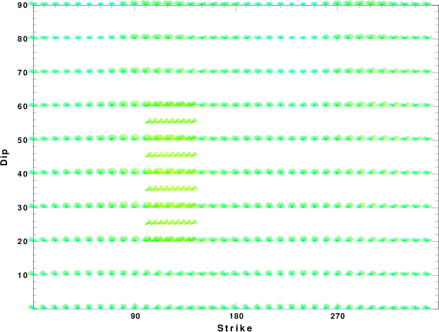
Focal mechanism sensitivity at the preferred depth. The red color indicates a very good fit to thewavefroms.
Each solution is plotted as a vector at a given value of strike and dip with the angle of the vector representing the rake angle, measured, with respect to the upward vertical (N) in the figure.
|
A check on the assumed source location is possible by looking at the time shifts between the observed and predicted traces. The time shifts for waveform matching arise for several reasons:
- The origin time and epicentral distance are incorrect
- The velocity model used for the inversion is incorrect
- The velocity model used to define the P-arrival time is not the
same as the velocity model used for the waveform inversion
(assuming that the initial trace alignment is based on the
P arrival time)
Assuming only a mislocation, the time shifts are fit to a functional form:
Time_shift = A + B cos Azimuth + C Sin Azimuth
The time shifts for this inversion lead to the next figure:
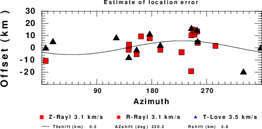
The derived shift in origin time and epicentral coordinates are given at the bottom of the figure.
Discussion
Velocity Model
The nnCIA used for the waveform synthetic seismograms and for the surface wave eigenfunctions and dispersion is as follows:
MODEL.01
C.It. A. Di Luzio et al Earth Plan Lettrs 280 (2009) 1-12 Fig 5. 7-8 MODEL/SURF3
ISOTROPIC
KGS
FLAT EARTH
1-D
CONSTANT VELOCITY
LINE08
LINE09
LINE10
LINE11
      H(KM)   VP(KM/S)   VS(KM/S) RHO(GM/CC)         QP         QS       ETAP       ETAS      FREFP      FREFS
     1.5000     3.7497     2.1436     2.2753  0.500E-02  0.100E-01   0.00       0.00       1.00       1.00
     3.0000     4.9399     2.8210     2.4858  0.500E-02  0.100E-01   0.00       0.00       1.00       1.00
     3.0000     6.0129     3.4336     2.7058  0.500E-02  0.100E-01   0.00       0.00       1.00       1.00
     7.0000     5.5516     3.1475     2.6093  0.167E-02  0.333E-02   0.00       0.00       1.00       1.00
    15.0000     5.8805     3.3583     2.6770  0.167E-02  0.333E-02   0.00       0.00       1.00       1.00
     6.0000     7.1059     4.0081     3.0002  0.167E-02  0.333E-02   0.00       0.00       1.00       1.00
     8.0000     7.1000     3.9864     3.0120  0.167E-02  0.333E-02   0.00       0.00       1.00       1.00
     0.0000     7.9000     4.4036     3.2760  0.167E-02  0.333E-02   0.00       0.00       1.00       1.00
Quality Control
Here we tabulate the reasons for not using certain digital data sets
The following stations did not have a valid response files:
DATE=Sun Nov 19 11:16:58 CST 2017
Last Changed 2017/11/19