Location
2016/10/26 17:10:36 42.8790 13.1290 9.3 5.40
 SLU Moment Tensor Solution
 ENS  2016/10/26 17:10:36:2  42.88   13.13   9.3 5.4

 Stations used:
   IV.ARVD IV.ATFO IV.ATPC IV.ATTE IV.ATVO IV.CAFI IV.CAMP
   IV.CERT IV.CESX IV.CING IV.FAGN IV.FIAM IV.GIGS IV.INTR
   IV.LATE IV.MCIV IV.MGAB IV.MTCE IV.PIEI IV.PTQR IV.SACS
   IV.SRES IV.T1243 IV.T1247

 Filtering commands used:
   cut o DIST/3.3 -20 o DIST/3.3 +50
   rtr
   taper w 0.1
   hp c 0.03 n 3
   lp c 0.10 n 3

 Best Fitting Double Couple
  Mo = 1.12e+24 dyne-cm
  Mw = 5.30
  Z  = 5 km
  Plane   Strike  Dip  Rake
   NP1      334    60   -93
   NP2      160    30   -85
  Principal Axes:
   Axis    Value   Plunge  Azimuth
    T   1.12e+24     15      66
    N   0.00e+00      2     336
    P  -1.12e+24     75     236

 Moment Tensor: (dyne-cm)
    Component   Value
       Mxx     1.45e+23
       Mxy     3.49e+23
       Mxz     2.71e+23
       Myy     8.23e+23
       Myz     4.96e+23
       Mzz    -9.68e+23


                     ##############
                 ##---#################
              ###--------#################
             ###-----------################
           ####--------------################
          ####-----------------###############
         ####-------------------###########   #
        #####--------------------########## T ##
        #####---------------------#########   ##
       ######----------------------##############
       ######-----------------------#############
       ######----------   -----------############
       #######--------- P -----------############
        ######---------   ------------##########
        #######-----------------------##########
         #######----------------------#########
          #######---------------------########
           #######--------------------#######
             #######------------------#####
              ########----------------####
                 ########------------##
                     ###########---


 Global CMT Convention Moment Tensor:
      R          T          P
 -9.68e+23   2.71e+23  -4.96e+23
  2.71e+23   1.45e+23  -3.49e+23
 -4.96e+23  -3.49e+23   8.23e+23


Details of the solution is found at

http://www.eas.slu.edu/eqc/eqc_mt/MECH.IT/20161026171036/index.html
|
Preferred Solution
The preferred solution from an analysis of the surface-wave spectral amplitude radiation pattern, waveform inversion and first motion observations is
      STK = 160
      DIP = 30
     RAKE = -85
       MW = 5.30
       HS = 5.0
The waveform inversion is preferred.
Moment Tensor Comparison
The following compares this source inversion to others
| SLU |
GCMT |
USGSW |
 SLU Moment Tensor Solution
 ENS  2016/10/26 17:10:36:2  42.88   13.13   9.3 5.4

 Stations used:
   IV.ARVD IV.ATFO IV.ATPC IV.ATTE IV.ATVO IV.CAFI IV.CAMP
   IV.CERT IV.CESX IV.CING IV.FAGN IV.FIAM IV.GIGS IV.INTR
   IV.LATE IV.MCIV IV.MGAB IV.MTCE IV.PIEI IV.PTQR IV.SACS
   IV.SRES IV.T1243 IV.T1247

 Filtering commands used:
   cut o DIST/3.3 -20 o DIST/3.3 +50
   rtr
   taper w 0.1
   hp c 0.03 n 3
   lp c 0.10 n 3

 Best Fitting Double Couple
  Mo = 1.12e+24 dyne-cm
  Mw = 5.30
  Z  = 5 km
  Plane   Strike  Dip  Rake
   NP1      334    60   -93
   NP2      160    30   -85
  Principal Axes:
   Axis    Value   Plunge  Azimuth
    T   1.12e+24     15      66
    N   0.00e+00      2     336
    P  -1.12e+24     75     236

 Moment Tensor: (dyne-cm)
    Component   Value
       Mxx     1.45e+23
       Mxy     3.49e+23
       Mxz     2.71e+23
       Myy     8.23e+23
       Myz     4.96e+23
       Mzz    -9.68e+23


                     ##############
                 ##---#################
              ###--------#################
             ###-----------################
           ####--------------################
          ####-----------------###############
         ####-------------------###########   #
        #####--------------------########## T ##
        #####---------------------#########   ##
       ######----------------------##############
       ######-----------------------#############
       ######----------   -----------############
       #######--------- P -----------############
        ######---------   ------------##########
        #######-----------------------##########
         #######----------------------#########
          #######---------------------########
           #######--------------------#######
             #######------------------#####
              ########----------------####
                 ########------------##
                     ###########---


 Global CMT Convention Moment Tensor:
      R          T          P
 -9.68e+23   2.71e+23  -4.96e+23
  2.71e+23   1.45e+23  -3.49e+23
 -4.96e+23  -3.49e+23   8.23e+23


Details of the solution is found at

http://www.eas.slu.edu/eqc/eqc_mt/MECH.IT/20161026171036/index.html
|
October 26, 2016, CENTRAL ITALY, MW=5.5

Howard Koss

CENTROID-MOMENT-TENSOR  SOLUTION
GCMT EVENT:     C201610261710A
DATA: II IU CU G  IC DK GE LD KP
 MN
L.P.BODY WAVES:103S, 164C, T= 40
SURFACE WAVES: 156S, 297C, T= 50
TIMESTAMP:      Q-20161026204105
CENTROID LOCATION:
ORIGIN TIME:      17:10:40.5 0.1
LAT:42.82N 0.01;LON: 13.12E 0.01
DEP: 12.0  FIX;TRIANG HDUR:  1.4
MOMENT TENSOR: SCALE 10**24 D-CM
RR=-2.250 0.026; TT= 0.162 0.026
PP= 2.090 0.022; RT=-0.240 0.089
RP=-0.895 0.073; TP=-0.728 0.023
PRINCIPAL AXES:
1.(T) VAL=  2.463;PLG=10;AZM= 73
2.(N)       0.022;    11;    165
3.(P)      -2.483;    75;    305
BEST DBLE.COUPLE:M0= 2.47*10**24
NP1: STRIKE=150;DIP=37;SLIP=-109
NP2: STRIKE=353;DIP=55;SLIP= -76

            -----######
        #----------########
      ##------------#########
    ###--------------##########
   ###----------------##########
  ####-----------------#######
  ####------------------###### T
 #####--------   -------######   #
 #####-------- P -------##########
 ######-------   --------#########
 ######------------------#########
  ######----------------#########
  #######---------------#########
   ########-------------########
    ########-----------########
      #########--------######
        ###########---#####
            ########---
|
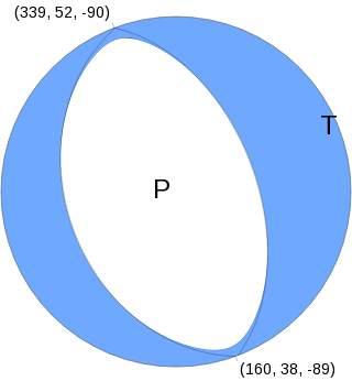
W-phase Moment Tensor (Mww)
Moment	2.430e+17 N-m
Magnitude	5.5 Mww
Depth	11.5 km
Percent DC	97 %
Half Duration	3 s
Catalog	US
Data Source	US1
Contributor	US1
Nodal Planes
Plane	Strike	Dip	Rake
NP1	160	38	-89
NP2	339	52	-90
Principal Axes
Axis	Value	Plunge	Azimuth
T	2.410e+17 N-m	7	70
N	0.038e+17 N-m	0	340
P	-2.448e+17 N-m	83	247
|
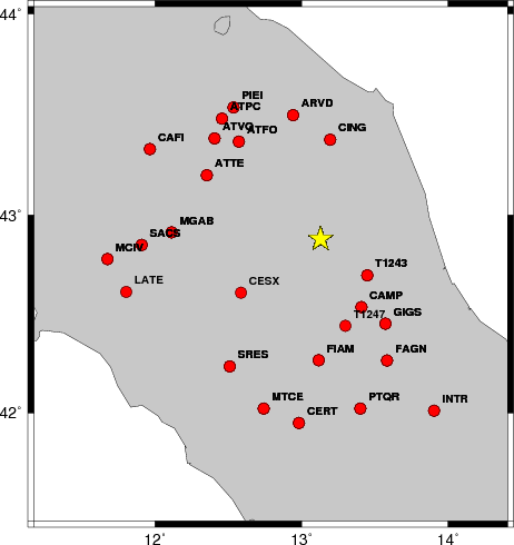
Waveform Inversion
The focal mechanism was determined using broadband seismic waveforms. The location of the event and the
and stations used for the waveform inversion are shown in the next figure.
|
|
Location of broadband stations used for waveform inversion
|
The program wvfgrd96 was used with good traces observed at short distance to determine the focal mechanism, depth and seismic moment. This technique requires a high quality signal and well determined velocity model for the Green functions. To the extent that these are the quality data, this type of mechanism should be preferred over the radiation pattern technique which requires the separate step of defining the pressure and tension quadrants and the correct strike.
The observed and predicted traces are filtered using the following gsac commands:
cut o DIST/3.3 -20 o DIST/3.3 +50
rtr
taper w 0.1
hp c 0.03 n 3
lp c 0.10 n 3
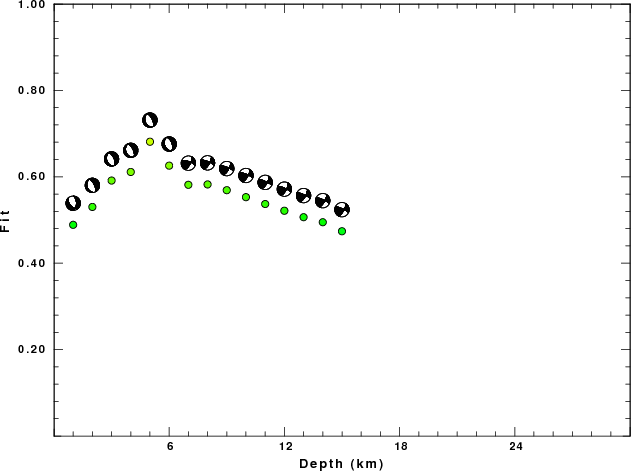
The results of this grid search from 0.5 to 19 km depth are as follow:
           DEPTH  STK   DIP  RAKE   MW    FIT
WVFGRD96    1.0     0    50   -60   5.06 0.4889
WVFGRD96    2.0   165    25   -80   5.18 0.5303
WVFGRD96    3.0   335    60   -95   5.20 0.5914
WVFGRD96    4.0   160    30   -85   5.21 0.6113
WVFGRD96    5.0   160    30   -85   5.30 0.6813
WVFGRD96    6.0   160    35   -90   5.29 0.6259
WVFGRD96    7.0    30    65    25   5.19 0.5816
WVFGRD96    8.0    30    65    20   5.19 0.5824
WVFGRD96    9.0    30    65    20   5.20 0.5691
WVFGRD96   10.0    30    65    20   5.20 0.5530
WVFGRD96   11.0    30    65    15   5.21 0.5371
WVFGRD96   12.0    30    65    15   5.22 0.5215
WVFGRD96   13.0    30    65    15   5.23 0.5066
WVFGRD96   14.0    30    65    15   5.24 0.4949
WVFGRD96   15.0    30    65    15   5.25 0.4740
The best solution is
WVFGRD96 5.0 160 30 -85 5.30 0.6813
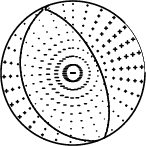
The mechanism correspond to the best fit is
|
|
Figure 1. Waveform inversion focal mechanism
|
The best fit as a function of depth is given in the following figure:
|
|
Figure 2. Depth sensitivity for waveform mechanism
|
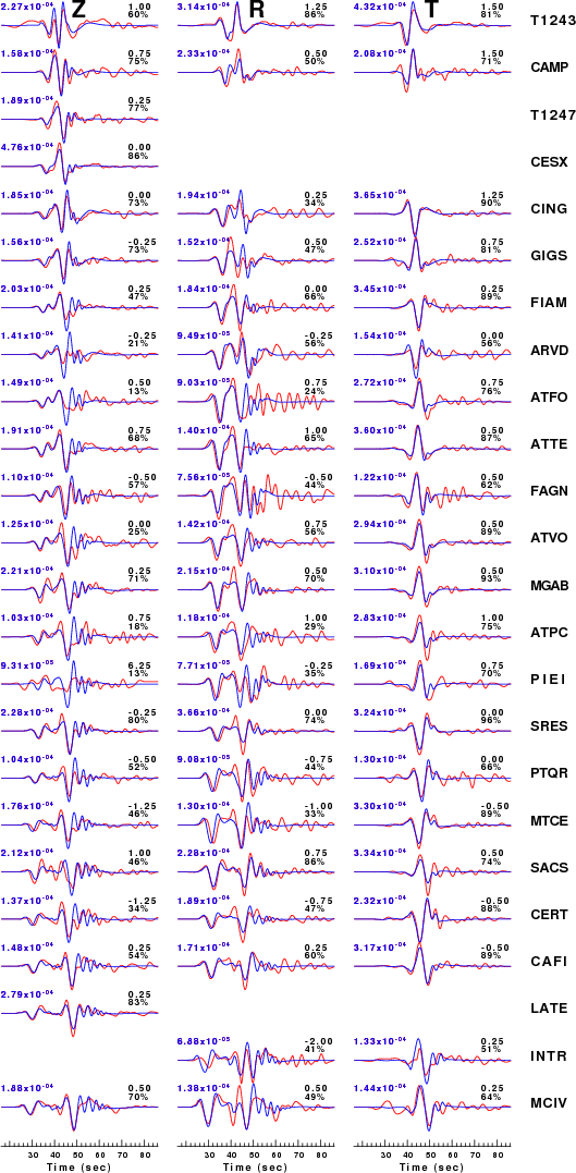
The comparison of the observed and predicted waveforms is given in the next figure. The red traces are the observed and the blue are the predicted.
Each observed-predicted component is plotted to the same scale and peak amplitudes are indicated by the numbers to the left of each trace. A pair of numbers is given in black at the right of each predicted traces. The upper number it the time shift required for maximum correlation between the observed and predicted traces. This time shift is required because the synthetics are not computed at exactly the same distance as the observed and because the velocity model used in the predictions may not be perfect.
A positive time shift indicates that the prediction is too fast and should be delayed to match the observed trace (shift to the right in this figure). A negative value indicates that the prediction is too slow. The lower number gives the percentage of variance reduction to characterize the individual goodness of fit (100% indicates a perfect fit).
The bandpass filter used in the processing and for the display was
cut o DIST/3.3 -20 o DIST/3.3 +50
rtr
taper w 0.1
hp c 0.03 n 3
lp c 0.10 n 3
|
|
Figure 3. Waveform comparison for selected depth. Red: observed; Blue - predicted. The time shift with respect to the model prediction is indicated. The percent of fit is also indicated.
|
|
|
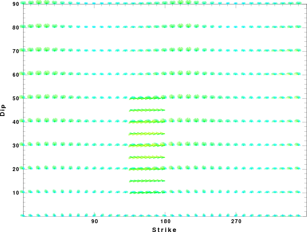
Focal mechanism sensitivity at the preferred depth. The red color indicates a very good fit to thewavefroms.
Each solution is plotted as a vector at a given value of strike and dip with the angle of the vector representing the rake angle, measured, with respect to the upward vertical (N) in the figure.
|
A check on the assumed source location is possible by looking at the time shifts between the observed and predicted traces. The time shifts for waveform matching arise for several reasons:
- The origin time and epicentral distance are incorrect
- The velocity model used for the inversion is incorrect
- The velocity model used to define the P-arrival time is not the
same as the velocity model used for the waveform inversion
(assuming that the initial trace alignment is based on the
P arrival time)
Assuming only a mislocation, the time shifts are fit to a functional form:
Time_shift = A + B cos Azimuth + C Sin Azimuth
The time shifts for this inversion lead to the next figure:
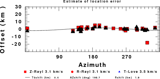
The derived shift in origin time and epicentral coordinates are given at the bottom of the figure.
Discussion
Velocity Model
The nnCIA used for the waveform synthetic seismograms and for the surface wave eigenfunctions and dispersion is as follows:
MODEL.01
C.It. A. Di Luzio et al Earth Plan Lettrs 280 (2009) 1-12 Fig 5. 7-8 MODEL/SURF3
ISOTROPIC
KGS
FLAT EARTH
1-D
CONSTANT VELOCITY
LINE08
LINE09
LINE10
LINE11
      H(KM)   VP(KM/S)   VS(KM/S) RHO(GM/CC)         QP         QS       ETAP       ETAS      FREFP      FREFS
     1.5000     3.7497     2.1436     2.2753  0.500E-02  0.100E-01   0.00       0.00       1.00       1.00
     3.0000     4.9399     2.8210     2.4858  0.500E-02  0.100E-01   0.00       0.00       1.00       1.00
     3.0000     6.0129     3.4336     2.7058  0.500E-02  0.100E-01   0.00       0.00       1.00       1.00
     7.0000     5.5516     3.1475     2.6093  0.167E-02  0.333E-02   0.00       0.00       1.00       1.00
    15.0000     5.8805     3.3583     2.6770  0.167E-02  0.333E-02   0.00       0.00       1.00       1.00
     6.0000     7.1059     4.0081     3.0002  0.167E-02  0.333E-02   0.00       0.00       1.00       1.00
     8.0000     7.1000     3.9864     3.0120  0.167E-02  0.333E-02   0.00       0.00       1.00       1.00
     0.0000     7.9000     4.4036     3.2760  0.167E-02  0.333E-02   0.00       0.00       1.00       1.00
Quality Control
Here we tabulate the reasons for not using certain digital data sets
The following stations did not have a valid response files:
DATE=Wed Oct 26 20:49:11 CDT 2016
Last Changed 2016/10/26