Location

2015/05/12 02:02:50 45.870 12.063 2.0 3.50 Italy

Arrival Times (from USGS)

Felt Map

Focal Mechanism

SLU Moment Tensor Solution ENS 2015/05/12 02:02:50:0 45.87 12.06 2.0 3.5 Italy Stations used: CH.BERNI CH.DAVOX IV.BRMO IV.CTI IV.PTCC IV.ROVR IV.STAL MN.TRI NI.ACOM NI.AGOR NI.SABO SI.LUSI SL.CADS SL.KNDS SL.ROBS SL.VOJS Filtering commands used: cut o DIST/3.3 -30 o DIST/3.3 +70 rtr taper w 0.1 hp c 0.02 n 3 lp c 0.06 n 3 Best Fitting Double Couple Mo = 1.38e+21 dyne-cm Mw = 3.36 Z = 8 km Plane Strike Dip Rake NP1 77 67 101 NP2 230 25 65 Principal Axes: Axis Value Plunge Azimuth T 1.38e+21 66 7 N 0.00e+00 10 253 P -1.38e+21 22 159 Moment Tensor: (dyne-cm) Component Value Mxx -8.05e+20 Mxy 4.29e+20 Mxz 9.56e+20 Myy -1.53e+20 Myz -1.12e+20 Mzz 9.58e+20 -------------- ---------------------- ----------################-- -------####################### -------########################### ------############################## -----############# ################# -----############## T ################## ----############### ################## ----####################################-- ----#################################----- ---################################------- ---############################----------- --#######################--------------- ##----##########------------------------ #------------------------------------- #----------------------------------- ---------------------------------- ------------------- -------- ------------------ P ------- --------------- ---- -------------- Global CMT Convention Moment Tensor: R T P 9.58e+20 9.56e+20 1.12e+20 9.56e+20 -8.05e+20 -4.29e+20 1.12e+20 -4.29e+20 -1.53e+20 Details of the solution is found at http://www.eas.slu.edu/eqc/eqc_mt/MECH.IT/20150512020250/index.html

Preferred Solution

The preferred solution from an analysis of the surface-wave spectral amplitude radiation pattern, waveform inversion and first motion observations is

      STK = 230
      DIP = 25
     RAKE = 65
       MW = 3.36
       HS = 8.0

The NDK file is 20150512020250.ndk The waveform inversion is preferred.

Moment Tensor Comparison

The following compares this source inversion to others

SLU

SLU Moment Tensor Solution ENS 2015/05/12 02:02:50:0 45.87 12.06 2.0 3.5 Italy Stations used: CH.BERNI CH.DAVOX IV.BRMO IV.CTI IV.PTCC IV.ROVR IV.STAL MN.TRI NI.ACOM NI.AGOR NI.SABO SI.LUSI SL.CADS SL.KNDS SL.ROBS SL.VOJS Filtering commands used: cut o DIST/3.3 -30 o DIST/3.3 +70 rtr taper w 0.1 hp c 0.02 n 3 lp c 0.06 n 3 Best Fitting Double Couple Mo = 1.38e+21 dyne-cm Mw = 3.36 Z = 8 km Plane Strike Dip Rake NP1 77 67 101 NP2 230 25 65 Principal Axes: Axis Value Plunge Azimuth T 1.38e+21 66 7 N 0.00e+00 10 253 P -1.38e+21 22 159 Moment Tensor: (dyne-cm) Component Value Mxx -8.05e+20 Mxy 4.29e+20 Mxz 9.56e+20 Myy -1.53e+20 Myz -1.12e+20 Mzz 9.58e+20 -------------- ---------------------- ----------################-- -------####################### -------########################### ------############################## -----############# ################# -----############## T ################## ----############### ################## ----####################################-- ----#################################----- ---################################------- ---############################----------- --#######################--------------- ##----##########------------------------ #------------------------------------- #----------------------------------- ---------------------------------- ------------------- -------- ------------------ P ------- --------------- ---- -------------- Global CMT Convention Moment Tensor: R T P 9.58e+20 9.56e+20 1.12e+20 9.56e+20 -8.05e+20 -4.29e+20 1.12e+20 -4.29e+20 -1.53e+20 Details of the solution is found at http://www.eas.slu.edu/eqc/eqc_mt/MECH.IT/20150512020250/index.html

Waveform Inversion

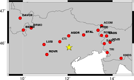
The focal mechanism was determined using broadband seismic waveforms. The location of the event and the and stations used for the waveform inversion are shown in the next figure.

Location of broadband stations used for waveform inversion

The program wvfgrd96 was used with good traces observed at short distance to determine the focal mechanism, depth and seismic moment. This technique requires a high quality signal and well determined velocity model for the Green functions. To the extent that these are the quality data, this type of mechanism should be preferred over the radiation pattern technique which requires the separate step of defining the pressure and tension quadrants and the correct strike.

The observed and predicted traces are filtered using the following gsac commands:

cut o DIST/3.3 -30 o DIST/3.3 +70
rtr
taper w 0.1
hp c 0.02 n 3 
lp c 0.06 n 3

The results of this grid search from 0.5 to 19 km depth are as follow:

           DEPTH  STK   DIP  RAKE   MW    FIT
WVFGRD96    1.0   200    75    20   3.12 0.3488
WVFGRD96    2.0   205    75    40   3.22 0.3519
WVFGRD96    3.0    25    80    55   3.26 0.3909
WVFGRD96    4.0    30    75    50   3.26 0.4264
WVFGRD96    5.0   220    15    45   3.40 0.4546
WVFGRD96    6.0   225    20    55   3.40 0.5047
WVFGRD96    7.0   230    20    65   3.41 0.5387
WVFGRD96    8.0   230    25    65   3.36 0.5589
WVFGRD96    9.0   230    25    65   3.35 0.5580
WVFGRD96   10.0   230    25    65   3.35 0.5499
WVFGRD96   11.0   225    25    60   3.34 0.5377
WVFGRD96   12.0   225    25    60   3.33 0.5235
WVFGRD96   13.0   225    25    60   3.33 0.5081
WVFGRD96   14.0   225    20    60   3.32 0.4924
WVFGRD96   15.0   225    20    60   3.36 0.4791
WVFGRD96   16.0   220    20    55   3.36 0.4629
WVFGRD96   17.0   220    20    55   3.36 0.4468
WVFGRD96   18.0   215    20    50   3.36 0.4308
WVFGRD96   19.0   215    20    50   3.36 0.4155
WVFGRD96   20.0   215    20    45   3.36 0.4003
WVFGRD96   21.0   215    20    45   3.36 0.3858
WVFGRD96   22.0   215    20    45   3.36 0.3717
WVFGRD96   23.0   215    20    45   3.36 0.3583
WVFGRD96   24.0   215    20    45   3.36 0.3451
WVFGRD96   25.0   210    25    40   3.36 0.3331
WVFGRD96   26.0   210    25    40   3.37 0.3224
WVFGRD96   27.0   210    25    40   3.37 0.3124
WVFGRD96   28.0   205    30    35   3.37 0.3030
WVFGRD96   29.0   205    30    35   3.37 0.2955

The best solution is

WVFGRD96    8.0   230    25    65   3.36 0.5589

The mechanism correspond to the best fit is

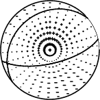
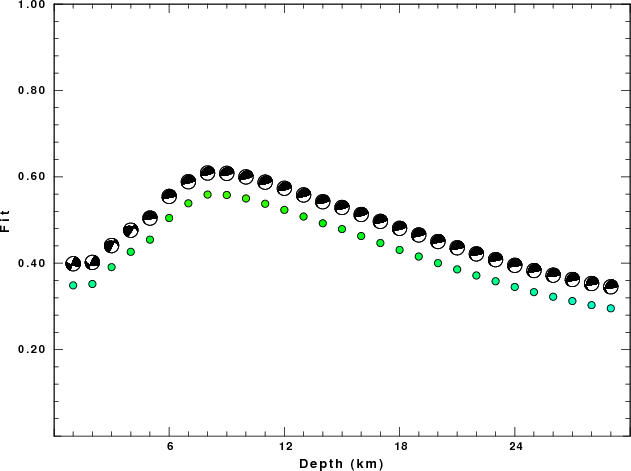
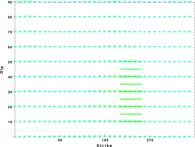
Figure 1. Waveform inversion focal mechanism

The best fit as a function of depth is given in the following figure:

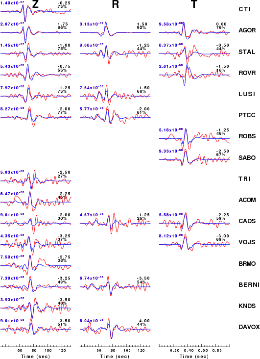
Figure 2. Depth sensitivity for waveform mechanism

The comparison of the observed and predicted waveforms is given in the next figure. The red traces are the observed and the blue are the predicted. Each observed-predicted component is plotted to the same scale and peak amplitudes are indicated by the numbers to the left of each trace. A pair of numbers is given in black at the right of each predicted traces. The upper number it the time shift required for maximum correlation between the observed and predicted traces. This time shift is required because the synthetics are not computed at exactly the same distance as the observed and because the velocity model used in the predictions may not be perfect. A positive time shift indicates that the prediction is too fast and should be delayed to match the observed trace (shift to the right in this figure). A negative value indicates that the prediction is too slow. The lower number gives the percentage of variance reduction to characterize the individual goodness of fit (100% indicates a perfect fit).

The bandpass filter used in the processing and for the display was

cut o DIST/3.3 -30 o DIST/3.3 +70
rtr
taper w 0.1
hp c 0.02 n 3 
lp c 0.06 n 3

Figure 3. Waveform comparison for selected depth. Red: observed; Blue - predicted. The time shift with respect to the model prediction is indicated. The percent of fit is also indicated.

Focal mechanism sensitivity at the preferred depth. The red color indicates a very good fit to thewavefroms. Each solution is plotted as a vector at a given value of strike and dip with the angle of the vector representing the rake angle, measured, with respect to the upward vertical (N) in the figure.

A check on the assumed source location is possible by looking at the time shifts between the observed and predicted traces. The time shifts for waveform matching arise for several reasons:

The origin time and epicentral distance are incorrect
The velocity model used for the inversion is incorrect
The velocity model used to define the P-arrival time is not the same as the velocity model used for the waveform inversion (assuming that the initial trace alignment is based on the P arrival time)

Assuming only a mislocation, the time shifts are fit to a functional form:

 Time_shift = A + B cos Azimuth + C Sin Azimuth

The time shifts for this inversion lead to the next figure:

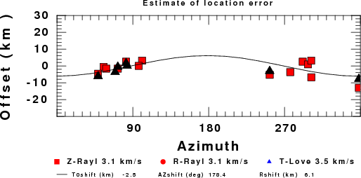
The derived shift in origin time and epicentral coordinates are given at the bottom of the figure.

Discussion

Velocity Model

The nnCIA used for the waveform synthetic seismograms and for the surface wave eigenfunctions and dispersion is as follows:

MODEL.01
C.It. A. Di Luzio et al Earth Plan Lettrs 280 (2009) 1-12 Fig 5. 7-8 MODEL/SURF3
ISOTROPIC
KGS
FLAT EARTH
1-D
CONSTANT VELOCITY
LINE08
LINE09
LINE10
LINE11
      H(KM)   VP(KM/S)   VS(KM/S) RHO(GM/CC)         QP         QS       ETAP       ETAS      FREFP      FREFS
     1.5000     3.7497     2.1436     2.2753  0.500E-02  0.100E-01   0.00       0.00       1.00       1.00    
     3.0000     4.9399     2.8210     2.4858  0.500E-02  0.100E-01   0.00       0.00       1.00       1.00    
     3.0000     6.0129     3.4336     2.7058  0.500E-02  0.100E-01   0.00       0.00       1.00       1.00    
     7.0000     5.5516     3.1475     2.6093  0.167E-02  0.333E-02   0.00       0.00       1.00       1.00    
    15.0000     5.8805     3.3583     2.6770  0.167E-02  0.333E-02   0.00       0.00       1.00       1.00    
     6.0000     7.1059     4.0081     3.0002  0.167E-02  0.333E-02   0.00       0.00       1.00       1.00    
     8.0000     7.1000     3.9864     3.0120  0.167E-02  0.333E-02   0.00       0.00       1.00       1.00    
     0.0000     7.9000     4.4036     3.2760  0.167E-02  0.333E-02   0.00       0.00       1.00       1.00

Quality Control

Here we tabulate the reasons for not using certain digital data sets

The following stations did not have a valid response files:

DATE=Tue May 12 15:30:49 CDT 2015

Last Changed 2015/05/12