Location

2014/07/21 11:12:28 42.113 15.877 7.0 3.30 Italy

Arrival Times (from USGS)

Felt Map

Focal Mechanism

SLU Moment Tensor Solution ENS 2014/07/21 11:12:28:0 42.11 15.88 7.0 3.3 Italy Stations used: IV.AMUR IV.BSSO IV.BULG IV.CAMP IV.CDRU IV.CERA IV.CIGN IV.CMPR IV.GATE IV.GUMA IV.INTR IV.LNSS IV.MCEL IV.MCRV IV.MELA IV.MGR IV.MIDA IV.MIGL IV.MOCO IV.MRVN IV.MSAG IV.MTSN IV.NOCI IV.PIGN IV.POFI IV.PTQR IV.SGG IV.SGRT IV.SIRI IV.SLCN IV.TERO IV.VAGA MN.AQU Filtering commands used: cut o DIST/3.3 -40 o DIST/3.3 +70 rtr taper w 0.1 hp c 0.03 n 3 lp c 0.10 n 3 Best Fitting Double Couple Mo = 8.22e+20 dyne-cm Mw = 3.21 Z = 18 km Plane Strike Dip Rake NP1 83 61 118 NP2 215 40 50 Principal Axes: Axis Value Plunge Azimuth T 8.22e+20 63 40 N 0.00e+00 24 248 P -8.22e+20 11 153 Moment Tensor: (dyne-cm) Component Value Mxx -5.23e+20 Mxy 4.08e+20 Mxz 3.94e+20 Myy -9.70e+19 Myz 1.43e+20 Mzz 6.20e+20 -------------- ---------------------- --------------############## ------------################## -----------####################### ----------########################## ----------############################ ---------############## ############## --------############### T ############## --------################ ############### --------################################-- -------###############################---- #------#############################------ ##---##########################--------- #####--###################-------------- ####---------------------------------- ####-------------------------------- ###------------------------------- ##-------------------- ----- #-------------------- P ---- ------------------ - -------------- Global CMT Convention Moment Tensor: R T P 6.20e+20 3.94e+20 -1.43e+20 3.94e+20 -5.23e+20 -4.08e+20 -1.43e+20 -4.08e+20 -9.70e+19 Details of the solution is found at http://www.eas.slu.edu/eqc/eqc_mt/MECH.IT/20140721111228/index.html

Preferred Solution

The preferred solution from an analysis of the surface-wave spectral amplitude radiation pattern, waveform inversion and first motion observations is

      STK = 215
      DIP = 40
     RAKE = 50
       MW = 3.21
       HS = 18.0

The NDK file is 20140721111228.ndk The waveform inversion is preferred.

Moment Tensor Comparison

The following compares this source inversion to others

SLU

SLU Moment Tensor Solution ENS 2014/07/21 11:12:28:0 42.11 15.88 7.0 3.3 Italy Stations used: IV.AMUR IV.BSSO IV.BULG IV.CAMP IV.CDRU IV.CERA IV.CIGN IV.CMPR IV.GATE IV.GUMA IV.INTR IV.LNSS IV.MCEL IV.MCRV IV.MELA IV.MGR IV.MIDA IV.MIGL IV.MOCO IV.MRVN IV.MSAG IV.MTSN IV.NOCI IV.PIGN IV.POFI IV.PTQR IV.SGG IV.SGRT IV.SIRI IV.SLCN IV.TERO IV.VAGA MN.AQU Filtering commands used: cut o DIST/3.3 -40 o DIST/3.3 +70 rtr taper w 0.1 hp c 0.03 n 3 lp c 0.10 n 3 Best Fitting Double Couple Mo = 8.22e+20 dyne-cm Mw = 3.21 Z = 18 km Plane Strike Dip Rake NP1 83 61 118 NP2 215 40 50 Principal Axes: Axis Value Plunge Azimuth T 8.22e+20 63 40 N 0.00e+00 24 248 P -8.22e+20 11 153 Moment Tensor: (dyne-cm) Component Value Mxx -5.23e+20 Mxy 4.08e+20 Mxz 3.94e+20 Myy -9.70e+19 Myz 1.43e+20 Mzz 6.20e+20 -------------- ---------------------- --------------############## ------------################## -----------####################### ----------########################## ----------############################ ---------############## ############## --------############### T ############## --------################ ############### --------################################-- -------###############################---- #------#############################------ ##---##########################--------- #####--###################-------------- ####---------------------------------- ####-------------------------------- ###------------------------------- ##-------------------- ----- #-------------------- P ---- ------------------ - -------------- Global CMT Convention Moment Tensor: R T P 6.20e+20 3.94e+20 -1.43e+20 3.94e+20 -5.23e+20 -4.08e+20 -1.43e+20 -4.08e+20 -9.70e+19 Details of the solution is found at http://www.eas.slu.edu/eqc/eqc_mt/MECH.IT/20140721111228/index.html

Waveform Inversion

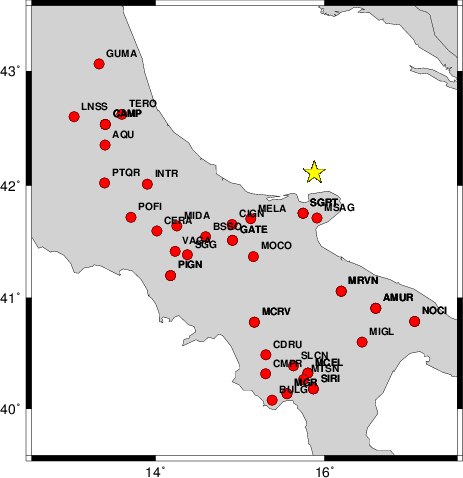
The focal mechanism was determined using broadband seismic waveforms. The location of the event and the and stations used for the waveform inversion are shown in the next figure.

Location of broadband stations used for waveform inversion

The program wvfgrd96 was used with good traces observed at short distance to determine the focal mechanism, depth and seismic moment. This technique requires a high quality signal and well determined velocity model for the Green functions. To the extent that these are the quality data, this type of mechanism should be preferred over the radiation pattern technique which requires the separate step of defining the pressure and tension quadrants and the correct strike.

The observed and predicted traces are filtered using the following gsac commands:

cut o DIST/3.3 -40 o DIST/3.3 +70
rtr
taper w 0.1
hp c 0.03 n 3 
lp c 0.10 n 3

The results of this grid search from 0.5 to 19 km depth are as follow:

           DEPTH  STK   DIP  RAKE   MW    FIT
WVFGRD96    1.0    95    45   -90   2.87 0.2286
WVFGRD96    2.0    95    45   -90   2.96 0.2272
WVFGRD96    3.0    35    80     5   2.92 0.1961
WVFGRD96    4.0    35    75     5   2.96 0.1929
WVFGRD96    5.0   210    45    -5   2.99 0.1915
WVFGRD96    6.0   205    40    10   2.99 0.2121
WVFGRD96    7.0   205    40    20   3.02 0.2412
WVFGRD96    8.0   205    40    30   3.01 0.2719
WVFGRD96    9.0   210    40    35   3.04 0.2977
WVFGRD96   10.0   210    40    40   3.06 0.3206
WVFGRD96   11.0   210    40    40   3.08 0.3399
WVFGRD96   12.0   210    40    40   3.09 0.3558
WVFGRD96   13.0   215    40    45   3.11 0.3688
WVFGRD96   14.0   215    40    45   3.13 0.3791
WVFGRD96   15.0   215    40    45   3.17 0.3879
WVFGRD96   16.0   215    40    45   3.19 0.3932
WVFGRD96   17.0   215    40    50   3.20 0.3961
WVFGRD96   18.0   215    40    50   3.21 0.3964
WVFGRD96   19.0   235    40    70   3.22 0.3949
WVFGRD96   20.0   240    40    80   3.23 0.3933
WVFGRD96   21.0    55    50    75   3.25 0.3916
WVFGRD96   22.0    55    50    75   3.26 0.3888
WVFGRD96   23.0    50    50    70   3.27 0.3833
WVFGRD96   24.0    50    50    70   3.28 0.3747
WVFGRD96   25.0    50    50    70   3.29 0.3638
WVFGRD96   26.0    50    50    70   3.29 0.3507
WVFGRD96   27.0    50    50    65   3.30 0.3362
WVFGRD96   28.0    45    50    65   3.32 0.3214
WVFGRD96   29.0    50    45    70   3.33 0.3072

The best solution is

WVFGRD96   18.0   215    40    50   3.21 0.3964

The mechanism correspond to the best fit is

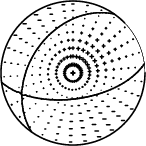
Figure 1. Waveform inversion focal mechanism

The best fit as a function of depth is given in the following figure:

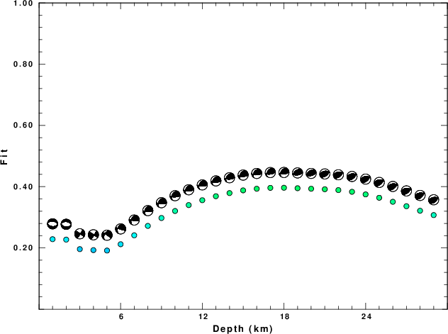
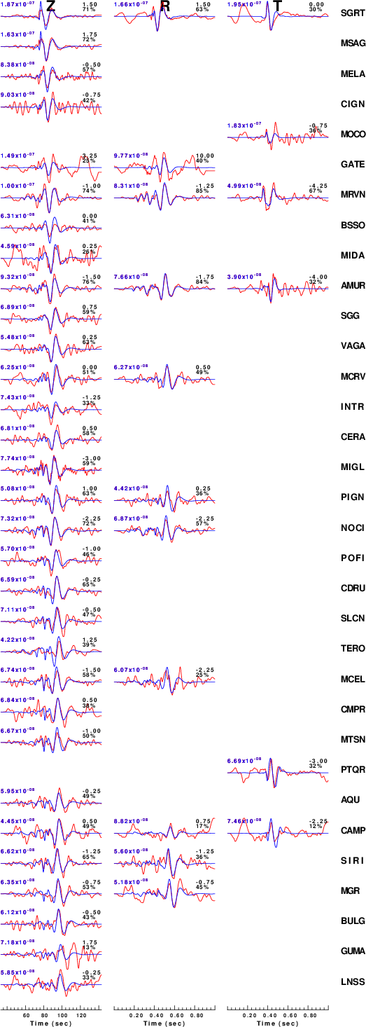
Figure 2. Depth sensitivity for waveform mechanism

The comparison of the observed and predicted waveforms is given in the next figure. The red traces are the observed and the blue are the predicted. Each observed-predicted component is plotted to the same scale and peak amplitudes are indicated by the numbers to the left of each trace. A pair of numbers is given in black at the right of each predicted traces. The upper number it the time shift required for maximum correlation between the observed and predicted traces. This time shift is required because the synthetics are not computed at exactly the same distance as the observed and because the velocity model used in the predictions may not be perfect. A positive time shift indicates that the prediction is too fast and should be delayed to match the observed trace (shift to the right in this figure). A negative value indicates that the prediction is too slow. The lower number gives the percentage of variance reduction to characterize the individual goodness of fit (100% indicates a perfect fit).

The bandpass filter used in the processing and for the display was

cut o DIST/3.3 -40 o DIST/3.3 +70
rtr
taper w 0.1
hp c 0.03 n 3 
lp c 0.10 n 3

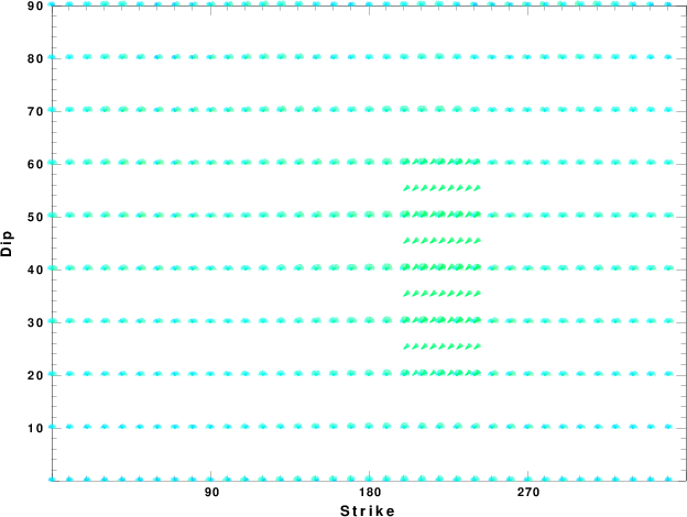
Figure 3. Waveform comparison for selected depth. Red: observed; Blue - predicted. The time shift with respect to the model prediction is indicated. The percent of fit is also indicated.

Focal mechanism sensitivity at the preferred depth. The red color indicates a very good fit to thewavefroms. Each solution is plotted as a vector at a given value of strike and dip with the angle of the vector representing the rake angle, measured, with respect to the upward vertical (N) in the figure.

A check on the assumed source location is possible by looking at the time shifts between the observed and predicted traces. The time shifts for waveform matching arise for several reasons:

The origin time and epicentral distance are incorrect
The velocity model used for the inversion is incorrect
The velocity model used to define the P-arrival time is not the same as the velocity model used for the waveform inversion (assuming that the initial trace alignment is based on the P arrival time)

Assuming only a mislocation, the time shifts are fit to a functional form:

 Time_shift = A + B cos Azimuth + C Sin Azimuth

The time shifts for this inversion lead to the next figure:

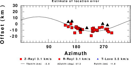
The derived shift in origin time and epicentral coordinates are given at the bottom of the figure.

Discussion

Velocity Model

The nnCIA used for the waveform synthetic seismograms and for the surface wave eigenfunctions and dispersion is as follows:

MODEL.01
C.It. A. Di Luzio et al Earth Plan Lettrs 280 (2009) 1-12 Fig 5. 7-8 MODEL/SURF3
ISOTROPIC
KGS
FLAT EARTH
1-D
CONSTANT VELOCITY
LINE08
LINE09
LINE10
LINE11
      H(KM)   VP(KM/S)   VS(KM/S) RHO(GM/CC)         QP         QS       ETAP       ETAS      FREFP      FREFS
     1.5000     3.7497     2.1436     2.2753  0.500E-02  0.100E-01   0.00       0.00       1.00       1.00    
     3.0000     4.9399     2.8210     2.4858  0.500E-02  0.100E-01   0.00       0.00       1.00       1.00    
     3.0000     6.0129     3.4336     2.7058  0.500E-02  0.100E-01   0.00       0.00       1.00       1.00    
     7.0000     5.5516     3.1475     2.6093  0.167E-02  0.333E-02   0.00       0.00       1.00       1.00    
    15.0000     5.8805     3.3583     2.6770  0.167E-02  0.333E-02   0.00       0.00       1.00       1.00    
     6.0000     7.1059     4.0081     3.0002  0.167E-02  0.333E-02   0.00       0.00       1.00       1.00    
     8.0000     7.1000     3.9864     3.0120  0.167E-02  0.333E-02   0.00       0.00       1.00       1.00    
     0.0000     7.9000     4.4036     3.2760  0.167E-02  0.333E-02   0.00       0.00       1.00       1.00

Quality Control

Here we tabulate the reasons for not using certain digital data sets

The following stations did not have a valid response files:

DATE=Mon Jul 21 17:15:38 CDT 2014

Last Changed 2014/07/21