Location
2014/01/20 07:12:40 41.362 14.449 11.1 4.20 Italy
Arrival Times (from USGS)
Arrival time list
Felt Map
USGS Felt map for this earthquake
USGS Felt reports page for
Focal Mechanism
 SLU Moment Tensor Solution
 ENS  2014/01/20 07:12:40:0  41.36   14.45  11.1 4.2 Italy

 Stations used:
   IV.BSSO IV.CDRU IV.CERA IV.CESX IV.CING IV.CMPR IV.FDMO
   IV.FRES IV.GATE IV.GIUL IV.INTR IV.LAV9 IV.LPEL IV.MCRV
   IV.MELA IV.MGR IV.MIDA IV.MOCO IV.MODR IV.MRLC IV.MRVN
   IV.MSAG IV.MTCE IV.NOCI IV.NRCA IV.PSB1 IV.RNI2 IV.ROM9
   IV.SACR IV.SGRT IV.SIRI IV.SLCN IV.SNAL IV.SNTG IV.T0104
   IV.TERO IV.VAGA IV.VVLD MN.AQU

 Filtering commands used:
   cut a -10 a 90
   rtr
   taper w 0.1
   hp c 0.02 n 3
   lp c 0.06 n 3

 Best Fitting Double Couple
  Mo = 2.60e+22 dyne-cm
  Mw = 4.21
  Z  = 15 km
  Plane   Strike  Dip  Rake
   NP1      325    65   -70
   NP2      104    32   -126
  Principal Axes:
   Axis    Value   Plunge  Azimuth
    T   2.60e+22     18      40
    N   0.00e+00     18     136
    P  -2.60e+22     64     269

 Moment Tensor: (dyne-cm)
    Component   Value
       Mxx     1.37e+22
       Mxy     1.16e+22
       Mxz     5.93e+21
       Myy     4.99e+21
       Myz     1.50e+22
       Mzz    -1.87e+22


                     ##############
                 ######################
              ------#################   ##
             ----------############## T ###
           ---------------###########   #####
          ------------------##################
         --------------------##################
        -----------------------#################
        -------------------------###############
       #--------------------------###############
       ##-----------   ------------##############
       ##----------- P -------------#############
       ###----------   --------------############
        ###---------------------------##########
        #####-------------------------#########-
         #####-------------------------#######-
          #######-----------------------####--
           #########--------------------#----
             ###########------------####---
              ##########################--
                 ######################
                     ##############


 Global CMT Convention Moment Tensor:
      R          T          P
 -1.87e+22   5.93e+21  -1.50e+22
  5.93e+21   1.37e+22  -1.16e+22
 -1.50e+22  -1.16e+22   4.99e+21


Details of the solution is found at

http://www.eas.slu.edu/eqc/eqc_mt/MECH.IT/20140120071240/index.html
|
Preferred Solution
The preferred solution from an analysis of the surface-wave spectral amplitude radiation pattern, waveform inversion and first motion observations is
      STK = 325
      DIP = 65
     RAKE = -70
       MW = 4.21
       HS = 15.0
The NDK file is 20140120071240.ndk
The waveform inversion is preferred.
Moment Tensor Comparison
The following compares this source inversion to others
| SLU |
INGVTDMT |
 SLU Moment Tensor Solution
 ENS  2014/01/20 07:12:40:0  41.36   14.45  11.1 4.2 Italy

 Stations used:
   IV.BSSO IV.CDRU IV.CERA IV.CESX IV.CING IV.CMPR IV.FDMO
   IV.FRES IV.GATE IV.GIUL IV.INTR IV.LAV9 IV.LPEL IV.MCRV
   IV.MELA IV.MGR IV.MIDA IV.MOCO IV.MODR IV.MRLC IV.MRVN
   IV.MSAG IV.MTCE IV.NOCI IV.NRCA IV.PSB1 IV.RNI2 IV.ROM9
   IV.SACR IV.SGRT IV.SIRI IV.SLCN IV.SNAL IV.SNTG IV.T0104
   IV.TERO IV.VAGA IV.VVLD MN.AQU

 Filtering commands used:
   cut a -10 a 90
   rtr
   taper w 0.1
   hp c 0.02 n 3
   lp c 0.06 n 3

 Best Fitting Double Couple
  Mo = 2.60e+22 dyne-cm
  Mw = 4.21
  Z  = 15 km
  Plane   Strike  Dip  Rake
   NP1      325    65   -70
   NP2      104    32   -126
  Principal Axes:
   Axis    Value   Plunge  Azimuth
    T   2.60e+22     18      40
    N   0.00e+00     18     136
    P  -2.60e+22     64     269

 Moment Tensor: (dyne-cm)
    Component   Value
       Mxx     1.37e+22
       Mxy     1.16e+22
       Mxz     5.93e+21
       Myy     4.99e+21
       Myz     1.50e+22
       Mzz    -1.87e+22


                     ##############
                 ######################
              ------#################   ##
             ----------############## T ###
           ---------------###########   #####
          ------------------##################
         --------------------##################
        -----------------------#################
        -------------------------###############
       #--------------------------###############
       ##-----------   ------------##############
       ##----------- P -------------#############
       ###----------   --------------############
        ###---------------------------##########
        #####-------------------------#########-
         #####-------------------------#######-
          #######-----------------------####--
           #########--------------------#----
             ###########------------####---
              ##########################--
                 ######################
                     ##############


 Global CMT Convention Moment Tensor:
      R          T          P
 -1.87e+22   5.93e+21  -1.50e+22
  5.93e+21   1.37e+22  -1.16e+22
 -1.50e+22  -1.16e+22   4.99e+21


Details of the solution is found at

http://www.eas.slu.edu/eqc/eqc_mt/MECH.IT/20140120071240/index.html
|
|
Waveform Inversion
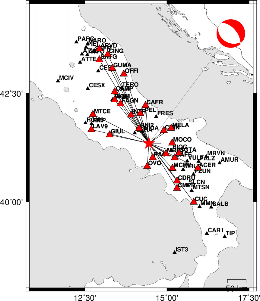
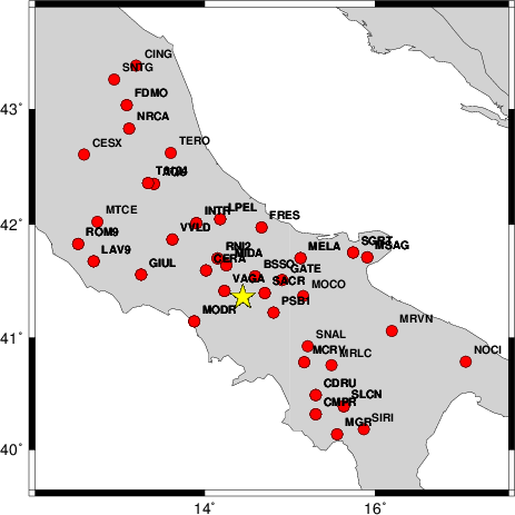
The focal mechanism was determined using broadband seismic waveforms. The location of the event and the
and stations used for the waveform inversion are shown in the next figure.
|
|
Location of broadband stations used for waveform inversion
|
The program wvfgrd96 was used with good traces observed at short distance to determine the focal mechanism, depth and seismic moment. This technique requires a high quality signal and well determined velocity model for the Green functions. To the extent that these are the quality data, this type of mechanism should be preferred over the radiation pattern technique which requires the separate step of defining the pressure and tension quadrants and the correct strike.
The observed and predicted traces are filtered using the following gsac commands:
cut a -10 a 90
rtr
taper w 0.1
hp c 0.02 n 3
lp c 0.06 n 3
The results of this grid search from 0.5 to 19 km depth are as follow:
           DEPTH  STK   DIP  RAKE   MW    FIT
WVFGRD96    1.0   350    40    80   3.92 0.2954
WVFGRD96    2.0   135    35   -90   4.06 0.2970
WVFGRD96    3.0   170    90    65   4.07 0.2943
WVFGRD96    4.0   350    90   -60   4.05 0.3285
WVFGRD96    5.0   340    85   -70   4.16 0.3604
WVFGRD96    6.0   335    80   -70   4.17 0.3964
WVFGRD96    7.0   320    75   -75   4.19 0.4367
WVFGRD96    8.0   320    70   -75   4.16 0.4734
WVFGRD96    9.0   315    65   -75   4.17 0.4980
WVFGRD96   10.0   320    65   -75   4.18 0.5171
WVFGRD96   11.0   320    65   -75   4.18 0.5306
WVFGRD96   12.0   320    65   -75   4.18 0.5389
WVFGRD96   13.0   320    65   -70   4.18 0.5435
WVFGRD96   14.0   320    65   -70   4.18 0.5456
WVFGRD96   15.0   325    65   -70   4.21 0.5514
WVFGRD96   16.0   325    65   -70   4.22 0.5486
WVFGRD96   17.0   325    65   -70   4.22 0.5438
WVFGRD96   18.0   325    65   -65   4.22 0.5377
WVFGRD96   19.0   325    65   -65   4.22 0.5304
WVFGRD96   20.0   325    65   -65   4.23 0.5216
WVFGRD96   21.0   330    65   -60   4.23 0.5118
WVFGRD96   22.0   330    65   -60   4.23 0.5018
WVFGRD96   23.0   330    65   -60   4.24 0.4909
WVFGRD96   24.0   330    65   -60   4.24 0.4804
WVFGRD96   25.0   330    65   -60   4.25 0.4697
WVFGRD96   26.0   325    65   -60   4.25 0.4578
WVFGRD96   27.0   325    65   -60   4.25 0.4459
WVFGRD96   28.0   325    65   -60   4.25 0.4334
WVFGRD96   29.0   325    65   -60   4.26 0.4212
The best solution is
WVFGRD96 15.0 325 65 -70 4.21 0.5514
The mechanism correspond to the best fit is
|
|
Figure 1. Waveform inversion focal mechanism
|
The best fit as a function of depth is given in the following figure:
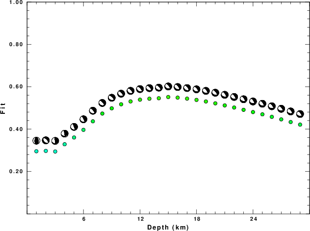
|
|
Figure 2. Depth sensitivity for waveform mechanism
|
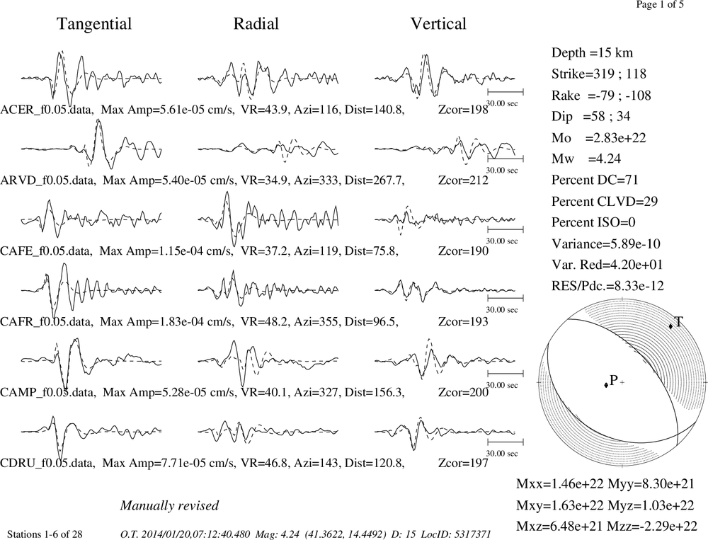
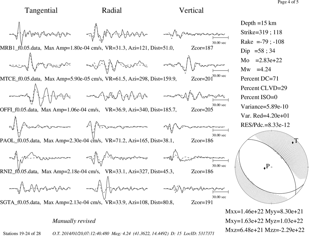
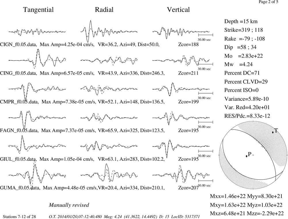
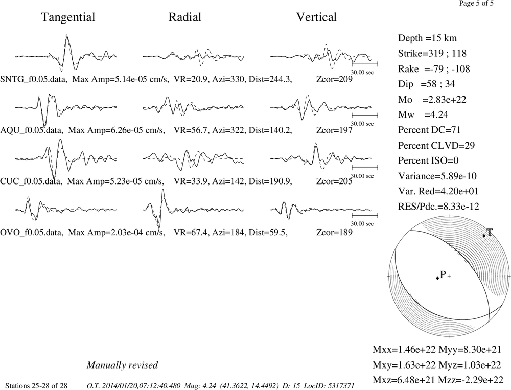
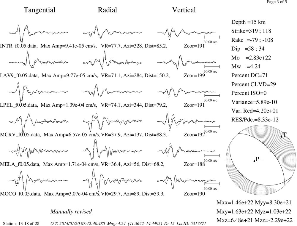
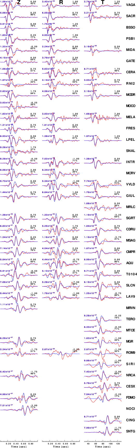
The comparison of the observed and predicted waveforms is given in the next figure. The red traces are the observed and the blue are the predicted.
Each observed-predicted component is plotted to the same scale and peak amplitudes are indicated by the numbers to the left of each trace. A pair of numbers is given in black at the right of each predicted traces. The upper number it the time shift required for maximum correlation between the observed and predicted traces. This time shift is required because the synthetics are not computed at exactly the same distance as the observed and because the velocity model used in the predictions may not be perfect.
A positive time shift indicates that the prediction is too fast and should be delayed to match the observed trace (shift to the right in this figure). A negative value indicates that the prediction is too slow. The lower number gives the percentage of variance reduction to characterize the individual goodness of fit (100% indicates a perfect fit).
The bandpass filter used in the processing and for the display was
cut a -10 a 90
rtr
taper w 0.1
hp c 0.02 n 3
lp c 0.06 n 3
|
|
Figure 3. Waveform comparison for selected depth. Red: observed; Blue - predicted. The time shift with respect to the model prediction is indicated. The percent of fit is also indicated.
|
|
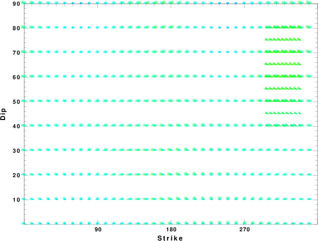
|
Focal mechanism sensitivity at the preferred depth. The red color indicates a very good fit to thewavefroms.
Each solution is plotted as a vector at a given value of strike and dip with the angle of the vector representing the rake angle, measured, with respect to the upward vertical (N) in the figure.
|
A check on the assumed source location is possible by looking at the time shifts between the observed and predicted traces. The time shifts for waveform matching arise for several reasons:
- The origin time and epicentral distance are incorrect
- The velocity model used for the inversion is incorrect
- The velocity model used to define the P-arrival time is not the
same as the velocity model used for the waveform inversion
(assuming that the initial trace alignment is based on the
P arrival time)
Assuming only a mislocation, the time shifts are fit to a functional form:
Time_shift = A + B cos Azimuth + C Sin Azimuth
The time shifts for this inversion lead to the next figure:
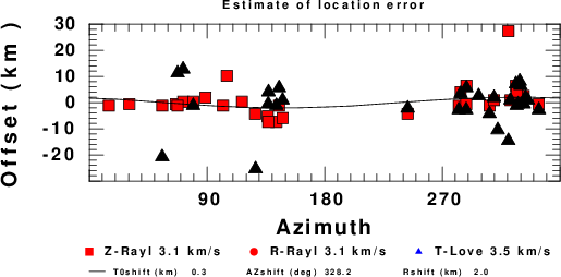
The derived shift in origin time and epicentral coordinates are given at the bottom of the figure.
Discussion
Velocity Model
The nnCIA used for the waveform synthetic seismograms and for the surface wave eigenfunctions and dispersion is as follows:
MODEL.01
C.It. A. Di Luzio et al Earth Plan Lettrs 280 (2009) 1-12 Fig 5. 7-8 MODEL/SURF3
ISOTROPIC
KGS
FLAT EARTH
1-D
CONSTANT VELOCITY
LINE08
LINE09
LINE10
LINE11
      H(KM)   VP(KM/S)   VS(KM/S) RHO(GM/CC)         QP         QS       ETAP       ETAS      FREFP      FREFS
     1.5000     3.7497     2.1436     2.2753  0.500E-02  0.100E-01   0.00       0.00       1.00       1.00
     3.0000     4.9399     2.8210     2.4858  0.500E-02  0.100E-01   0.00       0.00       1.00       1.00
     3.0000     6.0129     3.4336     2.7058  0.500E-02  0.100E-01   0.00       0.00       1.00       1.00
     7.0000     5.5516     3.1475     2.6093  0.167E-02  0.333E-02   0.00       0.00       1.00       1.00
    15.0000     5.8805     3.3583     2.6770  0.167E-02  0.333E-02   0.00       0.00       1.00       1.00
     6.0000     7.1059     4.0081     3.0002  0.167E-02  0.333E-02   0.00       0.00       1.00       1.00
     8.0000     7.1000     3.9864     3.0120  0.167E-02  0.333E-02   0.00       0.00       1.00       1.00
     0.0000     7.9000     4.4036     3.2760  0.167E-02  0.333E-02   0.00       0.00       1.00       1.00
Quality Control
Here we tabulate the reasons for not using certain digital data sets
The following stations did not have a valid response files:
DATE=Mon Jan 20 12:11:33 CST 2014
Last Changed 2014/01/20