Location
2013/12/29 17:08:43 41.37 14.45 10.5 4.90 Italy
Arrival Times (from USGS)
Arrival time list
Felt Map
USGS Felt map for this earthquake
USGS Felt reports page for
Focal Mechanism
 SLU Moment Tensor Solution
 ENS  2013/12/29 17:08:43:0  41.37   14.45  10.5 4.9 Italy

 Stations used:
   IV.ACER IV.AMUR IV.CAFR IV.CAMP IV.CDRU IV.CERA IV.CERT
   IV.CESI IV.CESX IV.CIGN IV.CING IV.CMPR IV.FDMO IV.FRES
   IV.GATE IV.GIUL IV.GUAR IV.GUMA IV.INTR IV.LAV9 IV.LNSS
   IV.LPEL IV.MA9 IV.MCEL IV.MCRV IV.MELA IV.MGR IV.MIDA
   IV.MIGL IV.MOCO IV.MODR IV.MRVN IV.MSAG IV.MTCE IV.MTSN
   IV.NOCI IV.NRCA IV.OFFI IV.PIGN IV.POFI IV.PSB1 IV.PTQR
   IV.RNI2 IV.SACR IV.SGRT IV.SIRI IV.SNAL IV.SNTG IV.T0104
   IV.TERO IV.TOLF IV.TRIV MN.AQU

 Filtering commands used:
   cut a -10 a 90
   rtr
   taper w 0.1
   hp c 0.02 n 3
   lp c 0.07 n 3

 Best Fitting Double Couple
  Mo = 4.12e+23 dyne-cm
  Mw = 5.01
  Z  = 15 km
  Plane   Strike  Dip  Rake
   NP1      330    60   -70
   NP2      114    36   -121
  Principal Axes:
   Axis    Value   Plunge  Azimuth
    T   4.12e+23     13      46
    N   0.00e+00     17     140
    P  -4.12e+23     68     281

 Moment Tensor: (dyne-cm)
    Component   Value
       Mxx     1.90e+23
       Mxy     2.06e+23
       Mxz     3.58e+22
       Myy     1.46e+23
       Myz     2.03e+23
       Mzz    -3.35e+23


                     ##############
                 --####################
              ---------###################
             -------------##############
           -----------------############ T ##
          --------------------##########   ###
         -----------------------###############
        #------------------------###############
        #-------------------------##############
       ##------------   -----------##############
       ###----------- P ------------#############
       ####----------   -------------############
       #####--------------------------###########
        #####-------------------------##########
        ######-------------------------#########
         #######-----------------------########
          #########--------------------######-
           ###########-----------------###---
             ##############----------##----
              #########################---
                 ######################
                     ##############


 Global CMT Convention Moment Tensor:
      R          T          P
 -3.35e+23   3.58e+22  -2.03e+23
  3.58e+22   1.90e+23  -2.06e+23
 -2.03e+23  -2.06e+23   1.46e+23


Details of the solution is found at

http://www.eas.slu.edu/eqc/eqc_mt/MECH.IT/20131229170843/index.html
|
Preferred Solution
The preferred solution from an analysis of the surface-wave spectral amplitude radiation pattern, waveform inversion and first motion observations is
      STK = 330
      DIP = 60
     RAKE = -70
       MW = 5.01
       HS = 15.0
The NDK file is 20131229170843.ndk
The waveform inversion is preferred.
Moment Tensor Comparison
The following compares this source inversion to others
| SLU |
USGSMT |
INGVTDMT |
 SLU Moment Tensor Solution
 ENS  2013/12/29 17:08:43:0  41.37   14.45  10.5 4.9 Italy

 Stations used:
   IV.ACER IV.AMUR IV.CAFR IV.CAMP IV.CDRU IV.CERA IV.CERT
   IV.CESI IV.CESX IV.CIGN IV.CING IV.CMPR IV.FDMO IV.FRES
   IV.GATE IV.GIUL IV.GUAR IV.GUMA IV.INTR IV.LAV9 IV.LNSS
   IV.LPEL IV.MA9 IV.MCEL IV.MCRV IV.MELA IV.MGR IV.MIDA
   IV.MIGL IV.MOCO IV.MODR IV.MRVN IV.MSAG IV.MTCE IV.MTSN
   IV.NOCI IV.NRCA IV.OFFI IV.PIGN IV.POFI IV.PSB1 IV.PTQR
   IV.RNI2 IV.SACR IV.SGRT IV.SIRI IV.SNAL IV.SNTG IV.T0104
   IV.TERO IV.TOLF IV.TRIV MN.AQU

 Filtering commands used:
   cut a -10 a 90
   rtr
   taper w 0.1
   hp c 0.02 n 3
   lp c 0.07 n 3

 Best Fitting Double Couple
  Mo = 4.12e+23 dyne-cm
  Mw = 5.01
  Z  = 15 km
  Plane   Strike  Dip  Rake
   NP1      330    60   -70
   NP2      114    36   -121
  Principal Axes:
   Axis    Value   Plunge  Azimuth
    T   4.12e+23     13      46
    N   0.00e+00     17     140
    P  -4.12e+23     68     281

 Moment Tensor: (dyne-cm)
    Component   Value
       Mxx     1.90e+23
       Mxy     2.06e+23
       Mxz     3.58e+22
       Myy     1.46e+23
       Myz     2.03e+23
       Mzz    -3.35e+23


                     ##############
                 --####################
              ---------###################
             -------------##############
           -----------------############ T ##
          --------------------##########   ###
         -----------------------###############
        #------------------------###############
        #-------------------------##############
       ##------------   -----------##############
       ###----------- P ------------#############
       ####----------   -------------############
       #####--------------------------###########
        #####-------------------------##########
        ######-------------------------#########
         #######-----------------------########
          #########--------------------######-
           ###########-----------------###---
             ##############----------##----
              #########################---
                 ######################
                     ##############


 Global CMT Convention Moment Tensor:
      R          T          P
 -3.35e+23   3.58e+22  -2.03e+23
  3.58e+22   1.90e+23  -2.06e+23
 -2.03e+23  -2.06e+23   1.46e+23


Details of the solution is found at

http://www.eas.slu.edu/eqc/eqc_mt/MECH.IT/20131229170843/index.html
|
Moment
    5.10e+16 N-m
Magnitude
    5.1
Percent DC
    77%
Depth
    14.0 km
Updated
    2013-12-29 20:24:44 UTC
Author
    us
Catalog
    us
Contributor
    us
Code
    us_c000ltr4_mwr

Principal Axes
Axis	Value	Plunge	Azimuth
T	5.374	2	42
N	-0.603	16	132
P	-4.771	73	304
Nodal Planes
Plane	Strike	Dip	Rake
NP1	327	49	-68
NP2	115	45	-113

|
|
Waveform Inversion
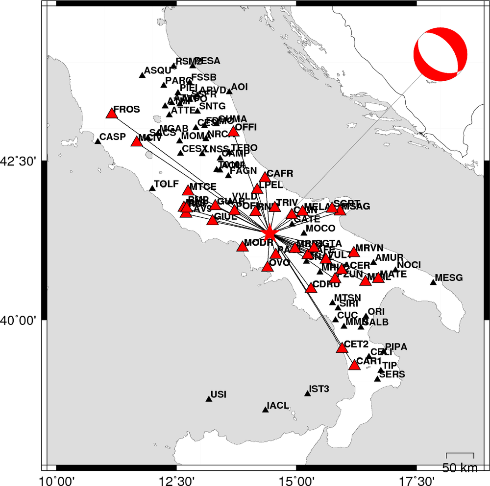
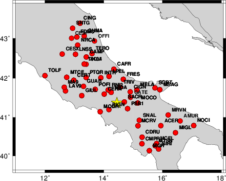
The focal mechanism was determined using broadband seismic waveforms. The location of the event and the
and stations used for the waveform inversion are shown in the next figure.
|
|
Location of broadband stations used for waveform inversion
|
The program wvfgrd96 was used with good traces observed at short distance to determine the focal mechanism, depth and seismic moment. This technique requires a high quality signal and well determined velocity model for the Green functions. To the extent that these are the quality data, this type of mechanism should be preferred over the radiation pattern technique which requires the separate step of defining the pressure and tension quadrants and the correct strike.
The observed and predicted traces are filtered using the following gsac commands:
cut a -10 a 90
rtr
taper w 0.1
hp c 0.02 n 3
lp c 0.07 n 3
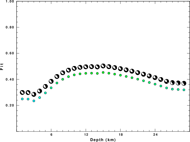
The results of this grid search from 0.5 to 19 km depth are as follow:
           DEPTH  STK   DIP  RAKE   MW    FIT
WVFGRD96    1.0   135    40   -90   4.78 0.2494
WVFGRD96    2.0   135    40   -90   4.84 0.2486
WVFGRD96    3.0   345    70   -55   4.83 0.2347
WVFGRD96    4.0   340    75   -60   4.84 0.2602
WVFGRD96    5.0   335    75   -70   4.95 0.2959
WVFGRD96    6.0   330    70   -75   4.97 0.3352
WVFGRD96    7.0   325    65   -75   4.98 0.3721
WVFGRD96    8.0   325    60   -75   4.96 0.4005
WVFGRD96    9.0   325    60   -75   4.96 0.4208
WVFGRD96   10.0   325    60   -75   4.97 0.4344
WVFGRD96   11.0   325    60   -75   4.97 0.4424
WVFGRD96   12.0   325    60   -75   4.97 0.4464
WVFGRD96   13.0   330    60   -70   4.97 0.4476
WVFGRD96   14.0   330    60   -70   4.98 0.4458
WVFGRD96   15.0   330    60   -70   5.01 0.4530
WVFGRD96   16.0   330    60   -70   5.02 0.4473
WVFGRD96   17.0   335    60   -65   5.02 0.4402
WVFGRD96   18.0   335    60   -60   5.02 0.4319
WVFGRD96   19.0   335    60   -60   5.03 0.4226
WVFGRD96   20.0   340    60   -55   5.03 0.4126
WVFGRD96   21.0   340    60   -55   5.04 0.4015
WVFGRD96   22.0   340    60   -55   5.04 0.3893
WVFGRD96   23.0   345    65   -45   5.05 0.3762
WVFGRD96   24.0   345    65   -45   5.05 0.3632
WVFGRD96   25.0   345    65   -45   5.06 0.3491
WVFGRD96   26.0   350    65   -40   5.07 0.3342
WVFGRD96   27.0   150    80    80   5.05 0.3251
WVFGRD96   28.0   150    80    75   5.05 0.3223
WVFGRD96   29.0   150    80    75   5.05 0.3196
The best solution is
WVFGRD96 15.0 330 60 -70 5.01 0.4530
The mechanism correspond to the best fit is
|
|
Figure 1. Waveform inversion focal mechanism
|
The best fit as a function of depth is given in the following figure:
|
|
Figure 2. Depth sensitivity for waveform mechanism
|
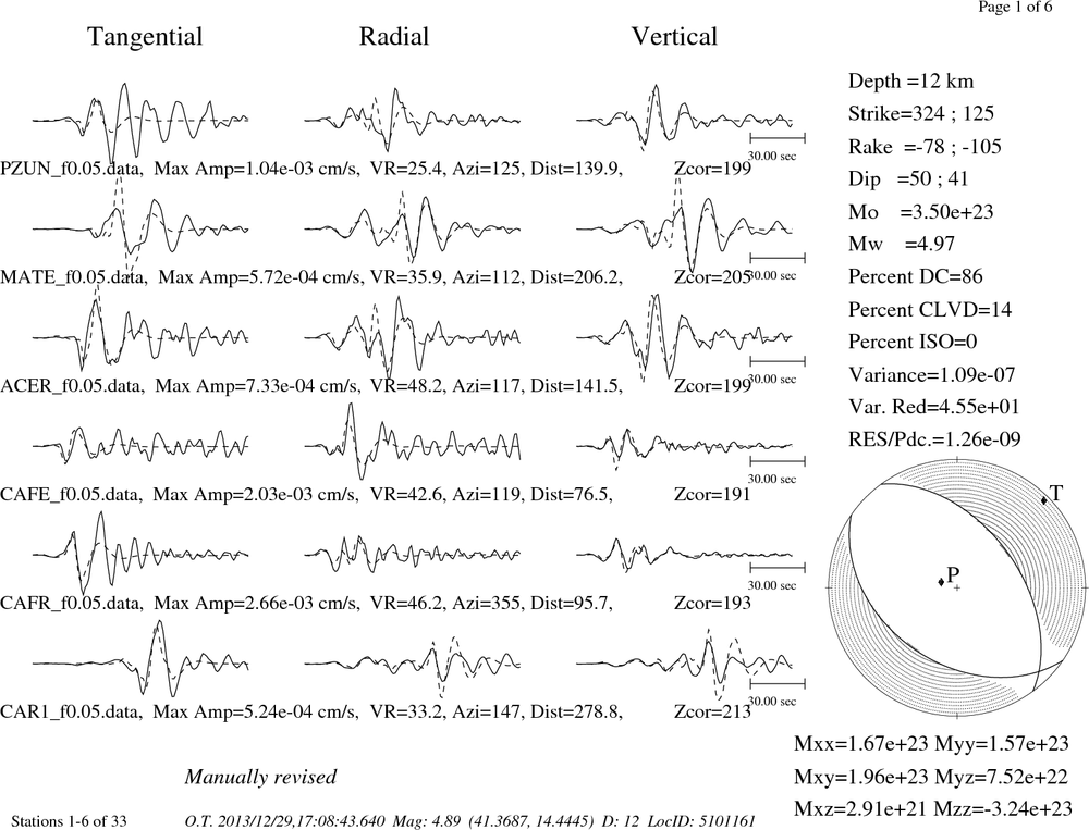
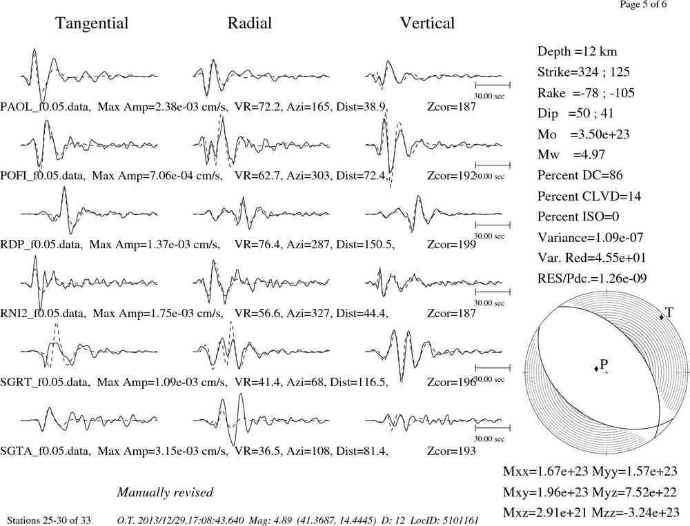
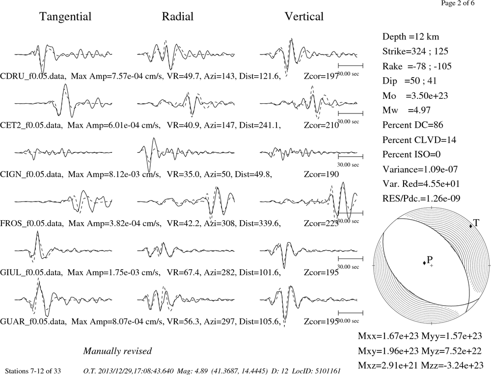
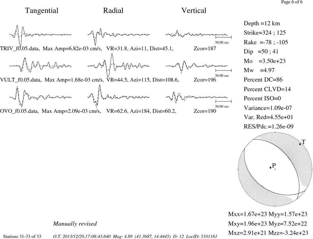
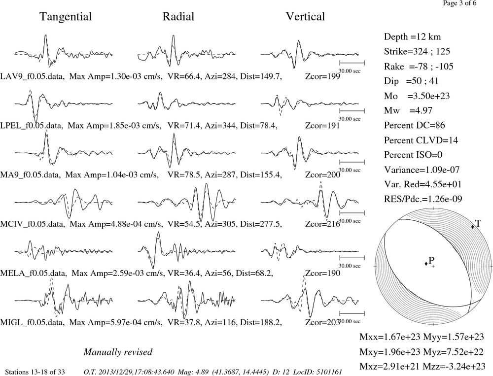
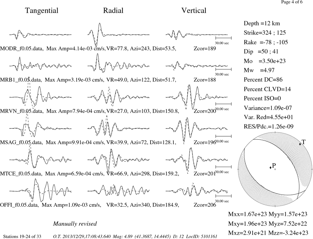
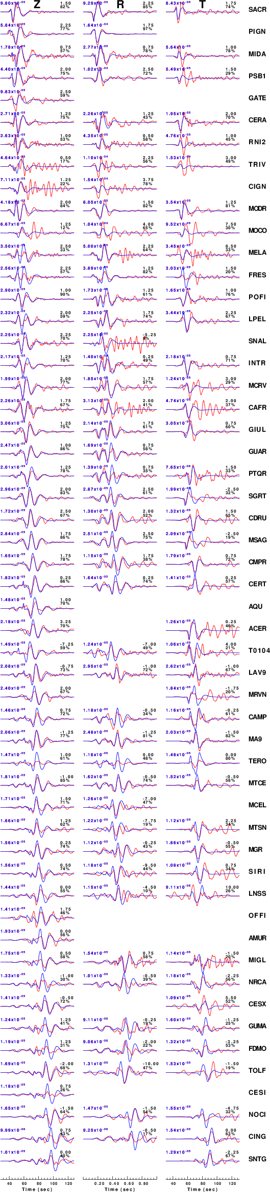
The comparison of the observed and predicted waveforms is given in the next figure. The red traces are the observed and the blue are the predicted.
Each observed-predicted component is plotted to the same scale and peak amplitudes are indicated by the numbers to the left of each trace. A pair of numbers is given in black at the right of each predicted traces. The upper number it the time shift required for maximum correlation between the observed and predicted traces. This time shift is required because the synthetics are not computed at exactly the same distance as the observed and because the velocity model used in the predictions may not be perfect.
A positive time shift indicates that the prediction is too fast and should be delayed to match the observed trace (shift to the right in this figure). A negative value indicates that the prediction is too slow. The lower number gives the percentage of variance reduction to characterize the individual goodness of fit (100% indicates a perfect fit).
The bandpass filter used in the processing and for the display was
cut a -10 a 90
rtr
taper w 0.1
hp c 0.02 n 3
lp c 0.07 n 3
|
|
Figure 3. Waveform comparison for selected depth. Red: observed; Blue - predicted. The time shift with respect to the model prediction is indicated. The percent of fit is also indicated.
|
|
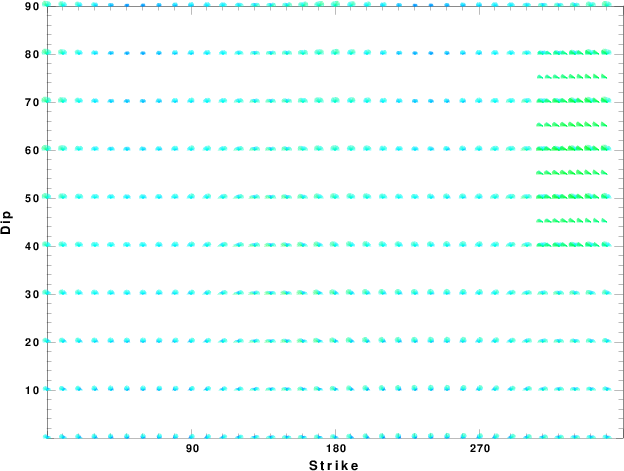
|
Focal mechanism sensitivity at the preferred depth. The red color indicates a very good fit to thewavefroms.
Each solution is plotted as a vector at a given value of strike and dip with the angle of the vector representing the rake angle, measured, with respect to the upward vertical (N) in the figure.
|
A check on the assumed source location is possible by looking at the time shifts between the observed and predicted traces. The time shifts for waveform matching arise for several reasons:
- The origin time and epicentral distance are incorrect
- The velocity model used for the inversion is incorrect
- The velocity model used to define the P-arrival time is not the
same as the velocity model used for the waveform inversion
(assuming that the initial trace alignment is based on the
P arrival time)
Assuming only a mislocation, the time shifts are fit to a functional form:
Time_shift = A + B cos Azimuth + C Sin Azimuth
The time shifts for this inversion lead to the next figure:
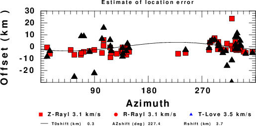
The derived shift in origin time and epicentral coordinates are given at the bottom of the figure.
Discussion
Velocity Model
The nnCIA used for the waveform synthetic seismograms and for the surface wave eigenfunctions and dispersion is as follows:
MODEL.01
C.It. A. Di Luzio et al Earth Plan Lettrs 280 (2009) 1-12 Fig 5. 7-8 MODEL/SURF3
ISOTROPIC
KGS
FLAT EARTH
1-D
CONSTANT VELOCITY
LINE08
LINE09
LINE10
LINE11
      H(KM)   VP(KM/S)   VS(KM/S) RHO(GM/CC)         QP         QS       ETAP       ETAS      FREFP      FREFS
     1.5000     3.7497     2.1436     2.2753  0.500E-02  0.100E-01   0.00       0.00       1.00       1.00
     3.0000     4.9399     2.8210     2.4858  0.500E-02  0.100E-01   0.00       0.00       1.00       1.00
     3.0000     6.0129     3.4336     2.7058  0.500E-02  0.100E-01   0.00       0.00       1.00       1.00
     7.0000     5.5516     3.1475     2.6093  0.167E-02  0.333E-02   0.00       0.00       1.00       1.00
    15.0000     5.8805     3.3583     2.6770  0.167E-02  0.333E-02   0.00       0.00       1.00       1.00
     6.0000     7.1059     4.0081     3.0002  0.167E-02  0.333E-02   0.00       0.00       1.00       1.00
     8.0000     7.1000     3.9864     3.0120  0.167E-02  0.333E-02   0.00       0.00       1.00       1.00
     0.0000     7.9000     4.4036     3.2760  0.167E-02  0.333E-02   0.00       0.00       1.00       1.00
Quality Control
Here we tabulate the reasons for not using certain digital data sets
The following stations did not have a valid response files:
DATE=Mon Dec 30 08:16:21 CST 2013
Last Changed 2013/12/29