Location

2013/10/19 12:29:35 43.675 10.274 9.9 3.40 Italy

Arrival Times (from USGS)

Felt Map

Focal Mechanism

SLU Moment Tensor Solution ENS 2013/10/19 12:29:35:0 43.67 10.27 9.9 3.4 Italy Stations used: FR.TURF GU.ENR GU.FINB GU.GORR GU.MAIM GU.PCP GU.POPM GU.STV IV.ARVD IV.ASQU IV.BDI IV.CAFI IV.CASP IV.CELB IV.CING IV.CRE IV.CRMI IV.FDMO IV.FNVD IV.GROG IV.MAON IV.MGAB IV.MSSA IV.MTRZ IV.MURB IV.PESA IV.PIEI IV.PLMA IV.QLNO IV.SACS IV.SNTG MN.VLC Filtering commands used: cut a -10 a 80 rtr taper w 0.1 hp c 0.02 n 3 lp c 0.10 n 3 Best Fitting Double Couple Mo = 2.16e+21 dyne-cm Mw = 3.49 Z = 6 km Plane Strike Dip Rake NP1 5 60 -50 NP2 126 48 -138 Principal Axes: Axis Value Plunge Azimuth T 2.16e+21 7 68 N 0.00e+00 34 162 P -2.16e+21 55 328 Moment Tensor: (dyne-cm) Component Value Mxx -1.98e+20 Mxy 1.06e+21 Mxz -7.65e+20 Myy 1.63e+21 Myz 7.65e+20 Mzz -1.43e+21 ----------#### ---------------####### -------------------######### ---------------------######### ------------------------########## #------------------------########### ##----------- ----------########## ###----------- P -----------######### T ####---------- -----------######### ######-----------------------############# #######----------------------############# ########---------------------############# #########-------------------############## ##########-----------------############# ###########----------------############# #############------------############# ###############--------############# #################-----############ ###################----------- #################----------- ############---------- #######------- Global CMT Convention Moment Tensor: R T P -1.43e+21 -7.65e+20 -7.65e+20 -7.65e+20 -1.98e+20 -1.06e+21 -7.65e+20 -1.06e+21 1.63e+21 Details of the solution is found at http://www.eas.slu.edu/eqc/eqc_mt/MECH.IT/20131019122935/index.html

Preferred Solution

The preferred solution from an analysis of the surface-wave spectral amplitude radiation pattern, waveform inversion and first motion observations is

      STK = 5
      DIP = 60
     RAKE = -50
       MW = 3.49
       HS = 6.0

The NDK file is 20131019122935.ndk The waveform inversion is preferred.

Moment Tensor Comparison

The following compares this source inversion to others

SLU

SLU Moment Tensor Solution ENS 2013/10/19 12:29:35:0 43.67 10.27 9.9 3.4 Italy Stations used: FR.TURF GU.ENR GU.FINB GU.GORR GU.MAIM GU.PCP GU.POPM GU.STV IV.ARVD IV.ASQU IV.BDI IV.CAFI IV.CASP IV.CELB IV.CING IV.CRE IV.CRMI IV.FDMO IV.FNVD IV.GROG IV.MAON IV.MGAB IV.MSSA IV.MTRZ IV.MURB IV.PESA IV.PIEI IV.PLMA IV.QLNO IV.SACS IV.SNTG MN.VLC Filtering commands used: cut a -10 a 80 rtr taper w 0.1 hp c 0.02 n 3 lp c 0.10 n 3 Best Fitting Double Couple Mo = 2.16e+21 dyne-cm Mw = 3.49 Z = 6 km Plane Strike Dip Rake NP1 5 60 -50 NP2 126 48 -138 Principal Axes: Axis Value Plunge Azimuth T 2.16e+21 7 68 N 0.00e+00 34 162 P -2.16e+21 55 328 Moment Tensor: (dyne-cm) Component Value Mxx -1.98e+20 Mxy 1.06e+21 Mxz -7.65e+20 Myy 1.63e+21 Myz 7.65e+20 Mzz -1.43e+21 ----------#### ---------------####### -------------------######### ---------------------######### ------------------------########## #------------------------########### ##----------- ----------########## ###----------- P -----------######### T ####---------- -----------######### ######-----------------------############# #######----------------------############# ########---------------------############# #########-------------------############## ##########-----------------############# ###########----------------############# #############------------############# ###############--------############# #################-----############ ###################----------- #################----------- ############---------- #######------- Global CMT Convention Moment Tensor: R T P -1.43e+21 -7.65e+20 -7.65e+20 -7.65e+20 -1.98e+20 -1.06e+21 -7.65e+20 -1.06e+21 1.63e+21 Details of the solution is found at http://www.eas.slu.edu/eqc/eqc_mt/MECH.IT/20131019122935/index.html

Waveform Inversion

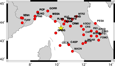
The focal mechanism was determined using broadband seismic waveforms. The location of the event and the and stations used for the waveform inversion are shown in the next figure.

Location of broadband stations used for waveform inversion

The program wvfgrd96 was used with good traces observed at short distance to determine the focal mechanism, depth and seismic moment. This technique requires a high quality signal and well determined velocity model for the Green functions. To the extent that these are the quality data, this type of mechanism should be preferred over the radiation pattern technique which requires the separate step of defining the pressure and tension quadrants and the correct strike.

The observed and predicted traces are filtered using the following gsac commands:

cut a -10 a 80
rtr
taper w 0.1
hp c 0.02 n 3 
lp c 0.10 n 3

The results of this grid search from 0.5 to 19 km depth are as follow:

           DEPTH  STK   DIP  RAKE   MW    FIT
WVFGRD96    1.0   290    75    10   3.17 0.2625
WVFGRD96    2.0   295    50    20   3.29 0.2854
WVFGRD96    3.0     5    60   -50   3.37 0.3510
WVFGRD96    4.0     0    55   -55   3.42 0.4049
WVFGRD96    5.0    -5    55   -65   3.51 0.4453
WVFGRD96    6.0     5    60   -50   3.49 0.4478
WVFGRD96    7.0    10    65   -40   3.48 0.4293
WVFGRD96    8.0    15    70   -35   3.46 0.4154
WVFGRD96    9.0    15    70   -30   3.47 0.4094
WVFGRD96   10.0    15    70   -30   3.48 0.4026
WVFGRD96   11.0    15    70   -30   3.49 0.3957
WVFGRD96   12.0    15    75   -30   3.50 0.3882
WVFGRD96   13.0    15    75   -30   3.51 0.3791
WVFGRD96   14.0    15    75   -25   3.52 0.3698
WVFGRD96   15.0    15    75   -30   3.54 0.3580
WVFGRD96   16.0    15    75   -30   3.55 0.3472
WVFGRD96   17.0    15    75   -30   3.56 0.3351
WVFGRD96   18.0    20    70    15   3.54 0.3206
WVFGRD96   19.0    20    70    15   3.55 0.3124
WVFGRD96   20.0    20    65    10   3.55 0.3050
WVFGRD96   21.0    20    65    10   3.56 0.2980
WVFGRD96   22.0    20    65    10   3.57 0.2922
WVFGRD96   23.0    25    60    20   3.57 0.2853
WVFGRD96   24.0   205    65    15   3.60 0.2840
WVFGRD96   25.0   205    65    10   3.60 0.2800
WVFGRD96   26.0   205    65    10   3.61 0.2764
WVFGRD96   27.0   200    70    10   3.63 0.2761
WVFGRD96   28.0   200    75    15   3.65 0.2740
WVFGRD96   29.0   200    80    15   3.68 0.2740

The best solution is

WVFGRD96    6.0     5    60   -50   3.49 0.4478

The mechanism correspond to the best fit is

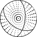
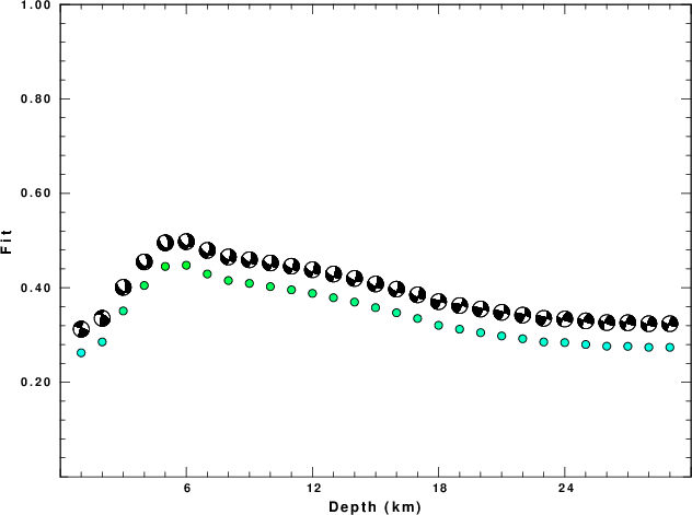
Figure 1. Waveform inversion focal mechanism

The best fit as a function of depth is given in the following figure:

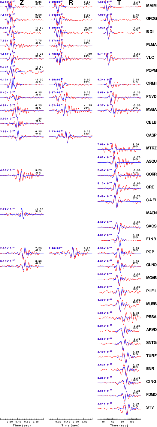
Figure 2. Depth sensitivity for waveform mechanism

The comparison of the observed and predicted waveforms is given in the next figure. The red traces are the observed and the blue are the predicted. Each observed-predicted component is plotted to the same scale and peak amplitudes are indicated by the numbers to the left of each trace. A pair of numbers is given in black at the right of each predicted traces. The upper number it the time shift required for maximum correlation between the observed and predicted traces. This time shift is required because the synthetics are not computed at exactly the same distance as the observed and because the velocity model used in the predictions may not be perfect. A positive time shift indicates that the prediction is too fast and should be delayed to match the observed trace (shift to the right in this figure). A negative value indicates that the prediction is too slow. The lower number gives the percentage of variance reduction to characterize the individual goodness of fit (100% indicates a perfect fit).

The bandpass filter used in the processing and for the display was

cut a -10 a 80
rtr
taper w 0.1
hp c 0.02 n 3 
lp c 0.10 n 3

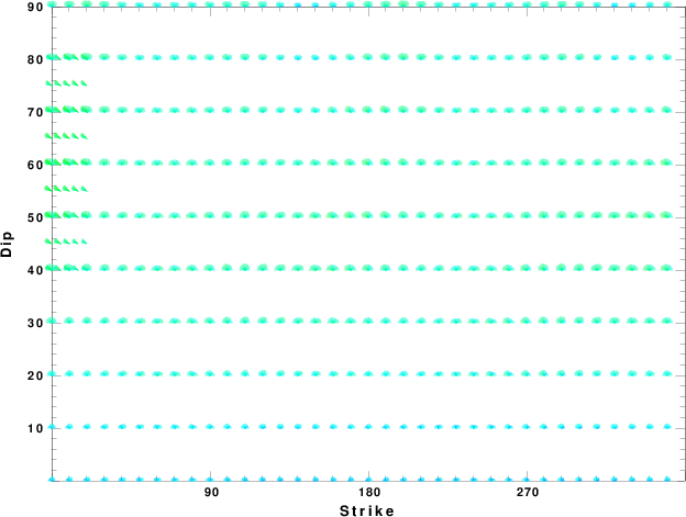
Figure 3. Waveform comparison for selected depth. Red: observed; Blue - predicted. The time shift with respect to the model prediction is indicated. The percent of fit is also indicated.

Focal mechanism sensitivity at the preferred depth. The red color indicates a very good fit to thewavefroms. Each solution is plotted as a vector at a given value of strike and dip with the angle of the vector representing the rake angle, measured, with respect to the upward vertical (N) in the figure.

A check on the assumed source location is possible by looking at the time shifts between the observed and predicted traces. The time shifts for waveform matching arise for several reasons:

The origin time and epicentral distance are incorrect
The velocity model used for the inversion is incorrect
The velocity model used to define the P-arrival time is not the same as the velocity model used for the waveform inversion (assuming that the initial trace alignment is based on the P arrival time)

Assuming only a mislocation, the time shifts are fit to a functional form:

 Time_shift = A + B cos Azimuth + C Sin Azimuth

The time shifts for this inversion lead to the next figure:

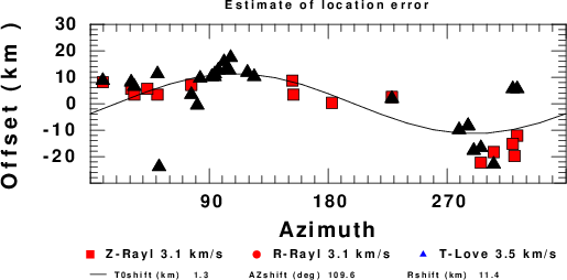
The derived shift in origin time and epicentral coordinates are given at the bottom of the figure.

Discussion

Velocity Model

The nnCIA used for the waveform synthetic seismograms and for the surface wave eigenfunctions and dispersion is as follows:

MODEL.01
C.It. A. Di Luzio et al Earth Plan Lettrs 280 (2009) 1-12 Fig 5. 7-8 MODEL/SURF3
ISOTROPIC
KGS
FLAT EARTH
1-D
CONSTANT VELOCITY
LINE08
LINE09
LINE10
LINE11
      H(KM)   VP(KM/S)   VS(KM/S) RHO(GM/CC)         QP         QS       ETAP       ETAS      FREFP      FREFS
     1.5000     3.7497     2.1436     2.2753  0.500E-02  0.100E-01   0.00       0.00       1.00       1.00    
     3.0000     4.9399     2.8210     2.4858  0.500E-02  0.100E-01   0.00       0.00       1.00       1.00    
     3.0000     6.0129     3.4336     2.7058  0.500E-02  0.100E-01   0.00       0.00       1.00       1.00    
     7.0000     5.5516     3.1475     2.6093  0.167E-02  0.333E-02   0.00       0.00       1.00       1.00    
    15.0000     5.8805     3.3583     2.6770  0.167E-02  0.333E-02   0.00       0.00       1.00       1.00    
     6.0000     7.1059     4.0081     3.0002  0.167E-02  0.333E-02   0.00       0.00       1.00       1.00    
     8.0000     7.1000     3.9864     3.0120  0.167E-02  0.333E-02   0.00       0.00       1.00       1.00    
     0.0000     7.9000     4.4036     3.2760  0.167E-02  0.333E-02   0.00       0.00       1.00       1.00

Quality Control

Here we tabulate the reasons for not using certain digital data sets

The following stations did not have a valid response files:

DATE=Sat Oct 19 09:53:42 CDT 2013

Last Changed 2013/10/19