Location
2013/08/22 06:44:50 43.583 13.804 7.9 4.4 Italy
Arrival Times (from USGS)
Arrival time list
Felt Map
USGS Felt map for this earthquake
USGS Felt reports page for
Focal Mechanism
 SLU Moment Tensor Solution
 ENS  2013/08/22 06:44:50:0  43.58   13.80   7.9 4.4 Italy

 Stations used:
   IV.ARVD IV.ASQU IV.CAFI IV.CERT IV.CESI IV.CESX IV.CING
   IV.FDMO IV.FIAM IV.FSSB IV.GUMA IV.LNSS IV.MGAB IV.MTCE
   IV.NRCA IV.PARC IV.PESA IV.PTQR IV.SACS IV.SNTG IV.SSFR
   IV.T0104 IV.TERO IV.VVLD

 Filtering commands used:
   cut a -10 a 80
   rtr
   taper w 0.1
   hp c 0.02 n 3
   lp c 0.05 n 3

 Best Fitting Double Couple
  Mo = 2.51e+22 dyne-cm
  Mw = 4.20
  Z  = 5 km
  Plane   Strike  Dip  Rake
   NP1      310    50    80
   NP2      145    41   102
  Principal Axes:
   Axis    Value   Plunge  Azimuth
    T   2.51e+22     81     167
    N   0.00e+00      8     316
    P  -2.51e+22      5      47

 Moment Tensor: (dyne-cm)
    Component   Value
       Mxx    -1.10e+22
       Mxy    -1.26e+22
       Mxz    -5.09e+21
       Myy    -1.34e+22
       Myz    -6.13e+20
       Mzz     2.44e+22


                     --------------
                 ----------------------
              #--------------------------
             #-#######------------------- P
           ---##############-------------   -
          ----#################---------------
         ----#####################-------------
        -----#######################------------
        ------########################----------
       -------#########################----------
       -------##########################---------
       --------############   ############-------
       ---------########### T ############-------
        ---------##########   #############-----
        ----------##########################----
         ----------#########################---
          -----------#######################--
           ------------#####################-
             ------------##################
              ---------------#############
                 ----------------------
                     --------------


 Global CMT Convention Moment Tensor:
      R          T          P
  2.44e+22  -5.09e+21   6.13e+20
 -5.09e+21  -1.10e+22   1.26e+22
  6.13e+20   1.26e+22  -1.34e+22


Details of the solution is found at

http://www.eas.slu.edu/eqc/eqc_mt/MECH.IT/20130822064450/index.html
|
Preferred Solution
The preferred solution from an analysis of the surface-wave spectral amplitude radiation pattern, waveform inversion and first motion observations is
      STK = 310
      DIP = 50
     RAKE = 80
       MW = 4.20
       HS = 5.0
The NDK file is 20130822064450.ndk
The waveform inversion is preferred.
Moment Tensor Comparison
The following compares this source inversion to others
| SLU |
INGVTDMT |
 SLU Moment Tensor Solution
 ENS  2013/08/22 06:44:50:0  43.58   13.80   7.9 4.4 Italy

 Stations used:
   IV.ARVD IV.ASQU IV.CAFI IV.CERT IV.CESI IV.CESX IV.CING
   IV.FDMO IV.FIAM IV.FSSB IV.GUMA IV.LNSS IV.MGAB IV.MTCE
   IV.NRCA IV.PARC IV.PESA IV.PTQR IV.SACS IV.SNTG IV.SSFR
   IV.T0104 IV.TERO IV.VVLD

 Filtering commands used:
   cut a -10 a 80
   rtr
   taper w 0.1
   hp c 0.02 n 3
   lp c 0.05 n 3

 Best Fitting Double Couple
  Mo = 2.51e+22 dyne-cm
  Mw = 4.20
  Z  = 5 km
  Plane   Strike  Dip  Rake
   NP1      310    50    80
   NP2      145    41   102
  Principal Axes:
   Axis    Value   Plunge  Azimuth
    T   2.51e+22     81     167
    N   0.00e+00      8     316
    P  -2.51e+22      5      47

 Moment Tensor: (dyne-cm)
    Component   Value
       Mxx    -1.10e+22
       Mxy    -1.26e+22
       Mxz    -5.09e+21
       Myy    -1.34e+22
       Myz    -6.13e+20
       Mzz     2.44e+22


                     --------------
                 ----------------------
              #--------------------------
             #-#######------------------- P
           ---##############-------------   -
          ----#################---------------
         ----#####################-------------
        -----#######################------------
        ------########################----------
       -------#########################----------
       -------##########################---------
       --------############   ############-------
       ---------########### T ############-------
        ---------##########   #############-----
        ----------##########################----
         ----------#########################---
          -----------#######################--
           ------------#####################-
             ------------##################
              ---------------#############
                 ----------------------
                     --------------


 Global CMT Convention Moment Tensor:
      R          T          P
  2.44e+22  -5.09e+21   6.13e+20
 -5.09e+21  -1.10e+22   1.26e+22
  6.13e+20   1.26e+22  -1.34e+22


Details of the solution is found at

http://www.eas.slu.edu/eqc/eqc_mt/MECH.IT/20130822064450/index.html
|
|
Waveform Inversion
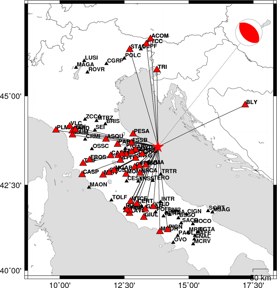
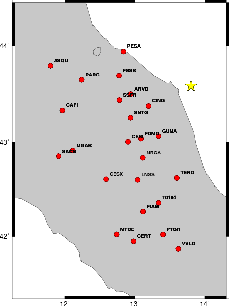
The focal mechanism was determined using broadband seismic waveforms. The location of the event and the
and stations used for the waveform inversion are shown in the next figure.
|
|
Location of broadband stations used for waveform inversion
|
The program wvfgrd96 was used with good traces observed at short distance to determine the focal mechanism, depth and seismic moment. This technique requires a high quality signal and well determined velocity model for the Green functions. To the extent that these are the quality data, this type of mechanism should be preferred over the radiation pattern technique which requires the separate step of defining the pressure and tension quadrants and the correct strike.
The observed and predicted traces are filtered using the following gsac commands:
cut a -10 a 80
rtr
taper w 0.1
hp c 0.02 n 3
lp c 0.05 n 3
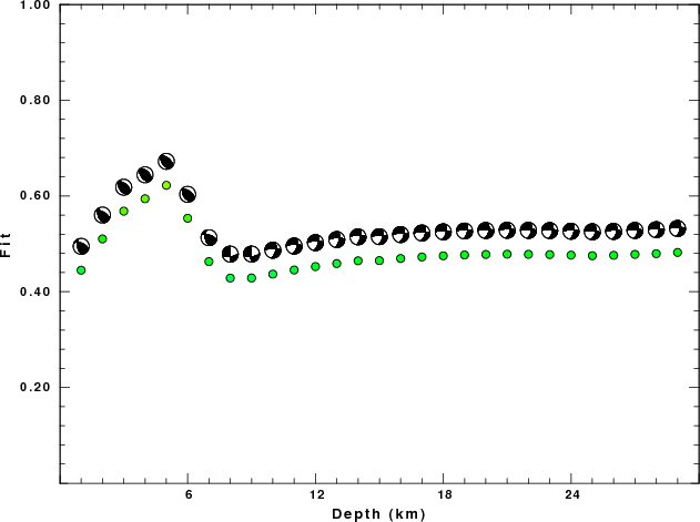
The results of this grid search from 0.5 to 19 km depth are as follow:
           DEPTH  STK   DIP  RAKE   MW    FIT
WVFGRD96    1.0   295    55    55   3.97 0.4449
WVFGRD96    2.0   300    55    65   4.04 0.5102
WVFGRD96    3.0   310    50    80   4.11 0.5683
WVFGRD96    4.0   315    45    85   4.16 0.5942
WVFGRD96    5.0   310    50    80   4.20 0.6223
WVFGRD96    6.0   305    50    75   4.20 0.5534
WVFGRD96    7.0   290    60    50   4.15 0.4629
WVFGRD96    8.0    85    60    -5   4.08 0.4286
WVFGRD96    9.0    85    60   -10   4.09 0.4287
WVFGRD96   10.0   270    70   -35   4.12 0.4367
WVFGRD96   11.0   270    70   -35   4.13 0.4454
WVFGRD96   12.0   270    70   -35   4.13 0.4525
WVFGRD96   13.0   270    70   -30   4.14 0.4589
WVFGRD96   14.0   270    70   -30   4.15 0.4646
WVFGRD96   15.0   270    75   -40   4.18 0.4650
WVFGRD96   16.0   270    75   -40   4.19 0.4694
WVFGRD96   17.0   270    75   -40   4.20 0.4726
WVFGRD96   18.0   270    75   -35   4.21 0.4750
WVFGRD96   19.0   270    75   -35   4.22 0.4768
WVFGRD96   20.0   270    75   -35   4.23 0.4779
WVFGRD96   21.0   270    75   -35   4.23 0.4784
WVFGRD96   22.0   270    75   -35   4.24 0.4782
WVFGRD96   23.0   270    75   -35   4.25 0.4776
WVFGRD96   24.0   270    75   -35   4.26 0.4764
WVFGRD96   25.0   275    80   -35   4.27 0.4752
WVFGRD96   26.0   270    75   -35   4.28 0.4760
WVFGRD96   27.0   270    75   -35   4.29 0.4780
WVFGRD96   28.0   270    75   -35   4.30 0.4795
WVFGRD96   29.0   270    75   -30   4.31 0.4821
The best solution is
WVFGRD96 5.0 310 50 80 4.20 0.6223
The mechanism correspond to the best fit is
|
|
Figure 1. Waveform inversion focal mechanism
|
The best fit as a function of depth is given in the following figure:
|
|
Figure 2. Depth sensitivity for waveform mechanism
|
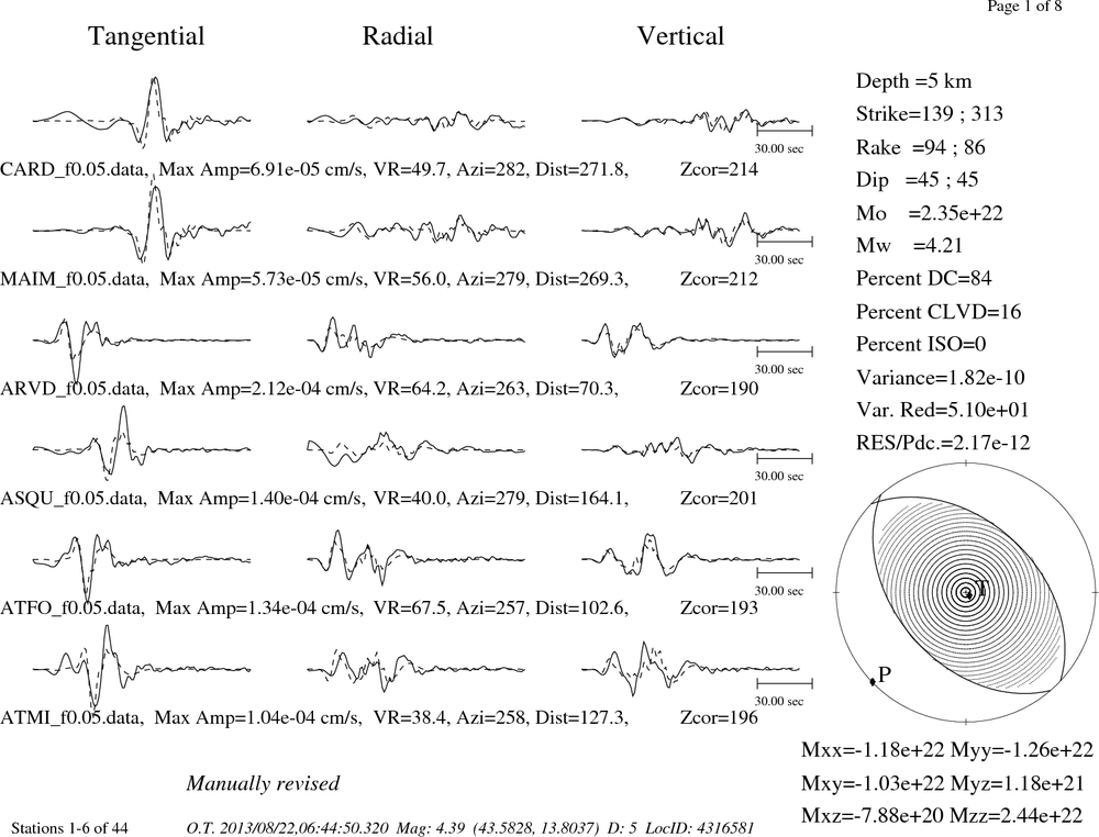
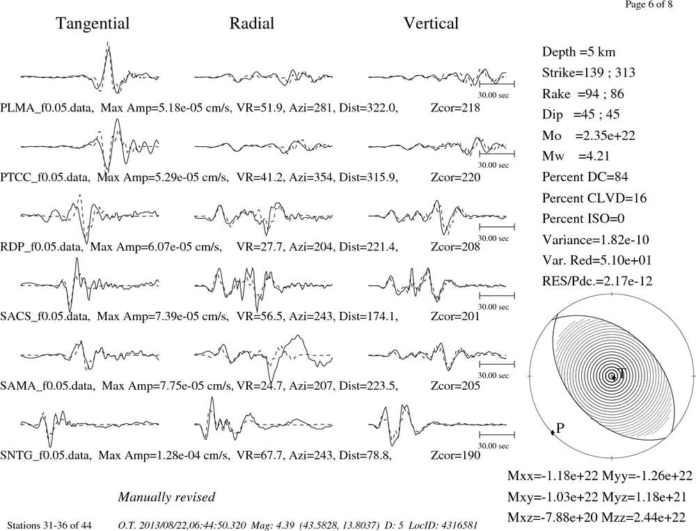
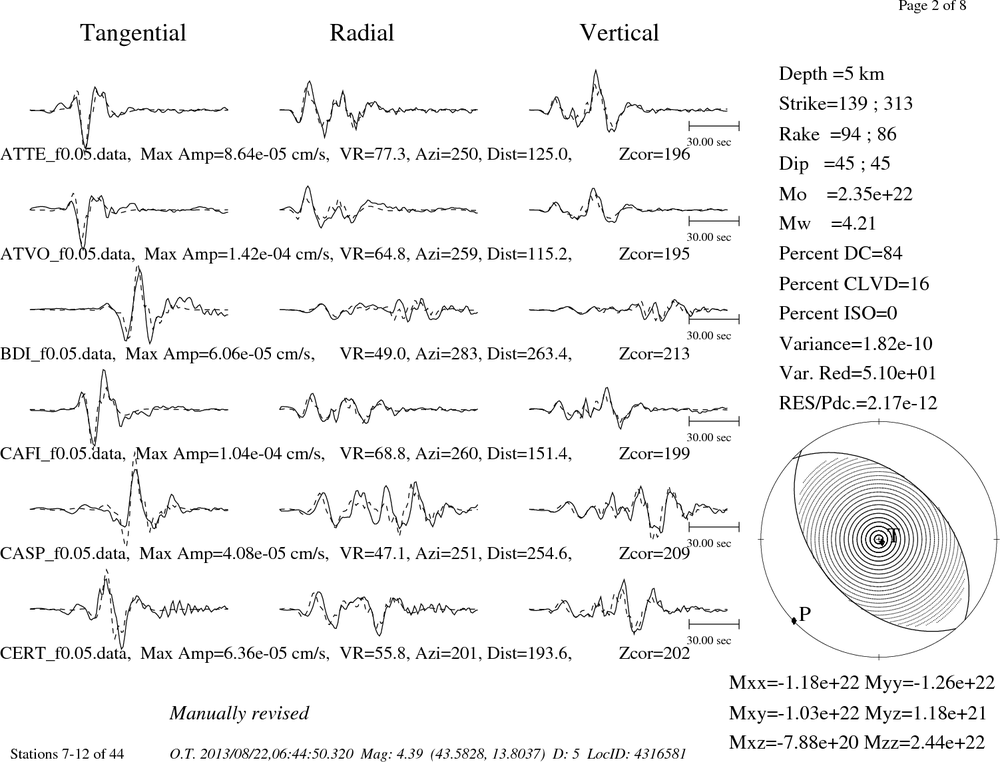
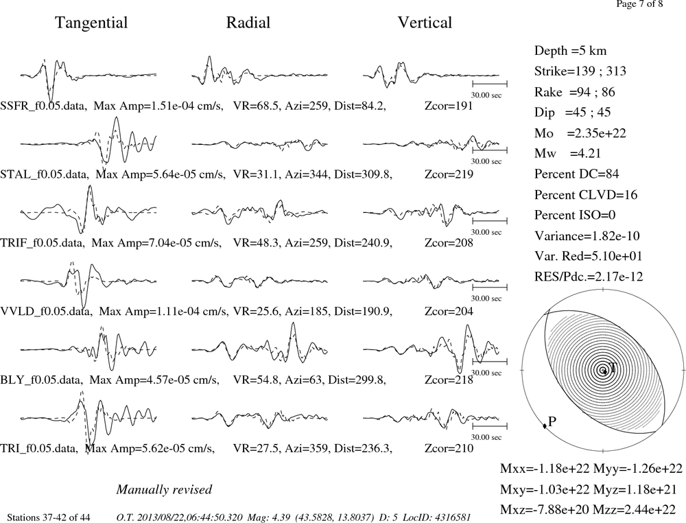
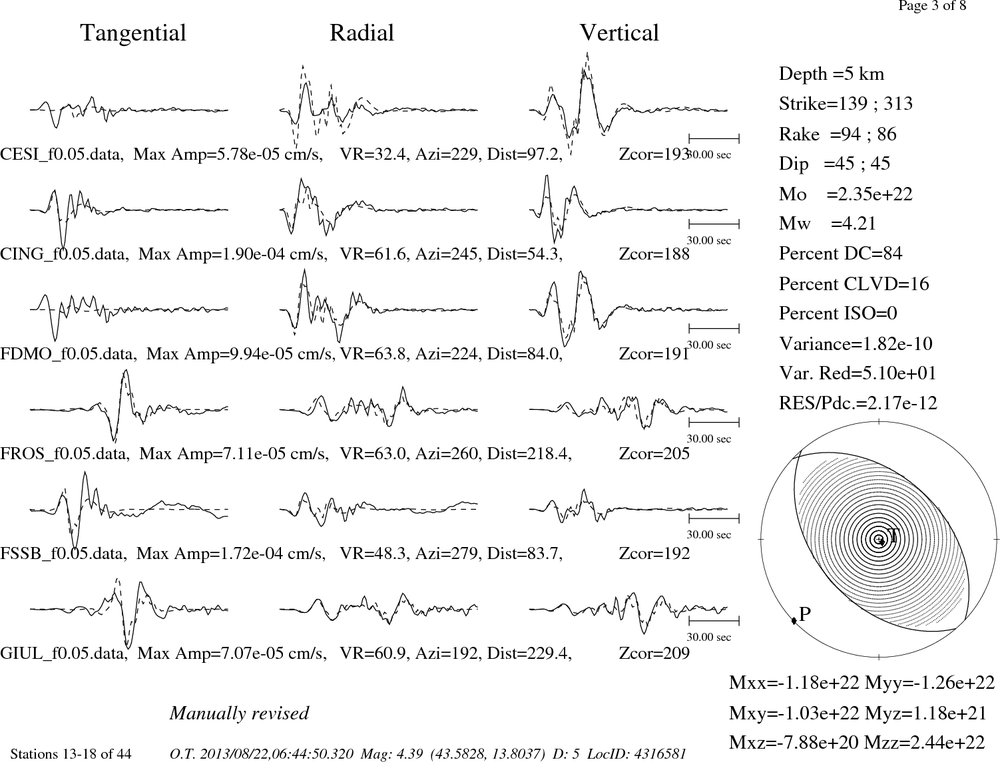
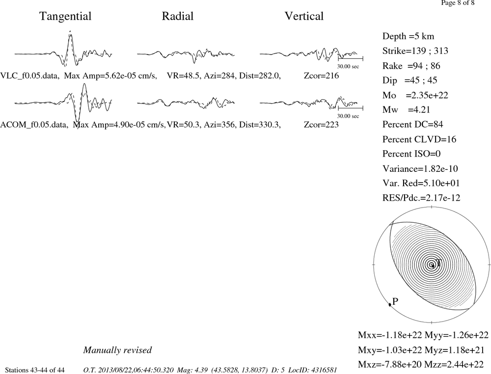
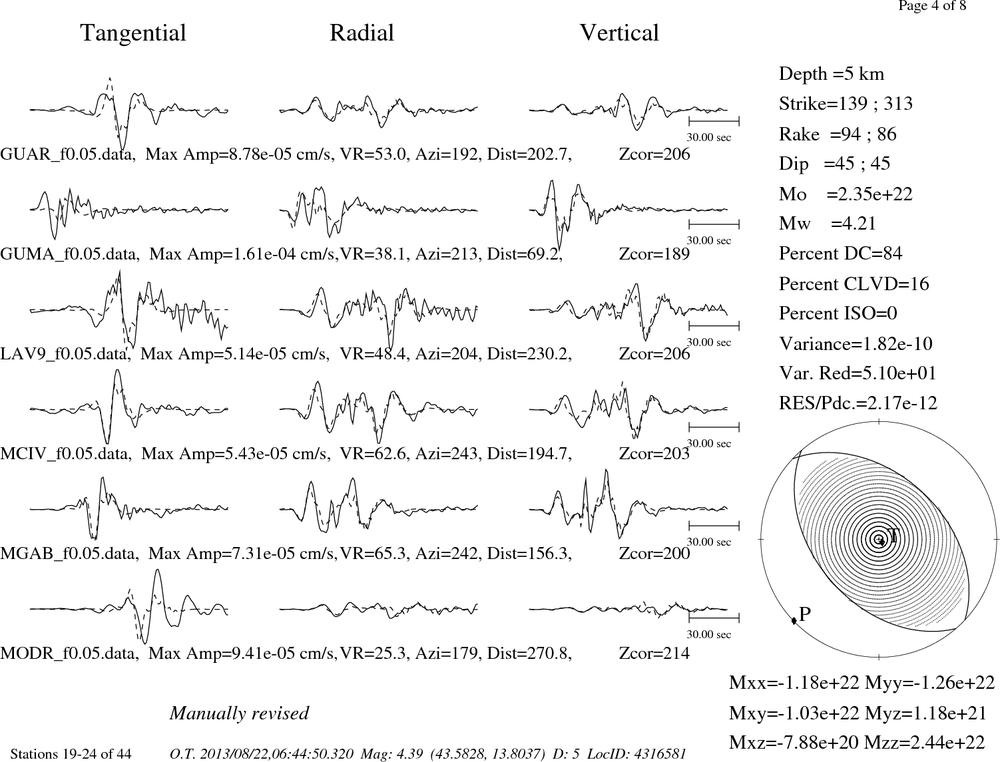
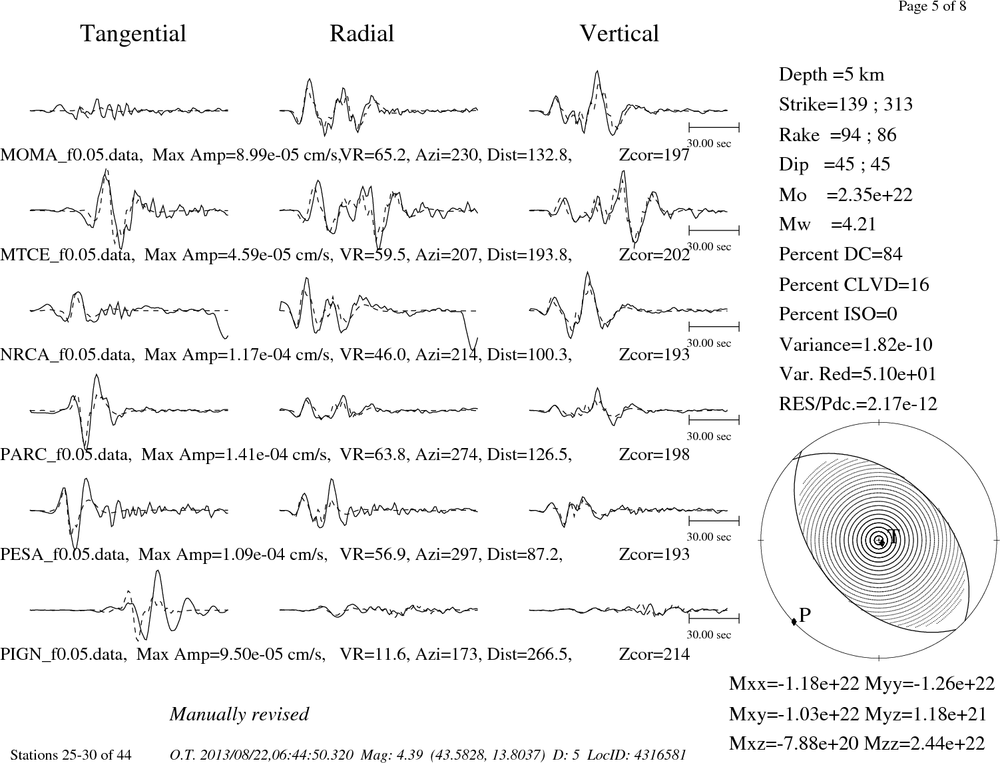
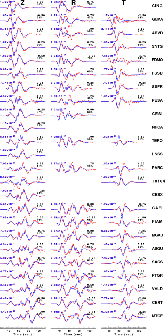
The comparison of the observed and predicted waveforms is given in the next figure. The red traces are the observed and the blue are the predicted.
Each observed-predicted component is plotted to the same scale and peak amplitudes are indicated by the numbers to the left of each trace. A pair of numbers is given in black at the right of each predicted traces. The upper number it the time shift required for maximum correlation between the observed and predicted traces. This time shift is required because the synthetics are not computed at exactly the same distance as the observed and because the velocity model used in the predictions may not be perfect.
A positive time shift indicates that the prediction is too fast and should be delayed to match the observed trace (shift to the right in this figure). A negative value indicates that the prediction is too slow. The lower number gives the percentage of variance reduction to characterize the individual goodness of fit (100% indicates a perfect fit).
The bandpass filter used in the processing and for the display was
cut a -10 a 80
rtr
taper w 0.1
hp c 0.02 n 3
lp c 0.05 n 3
|
|
Figure 3. Waveform comparison for selected depth
|
|
|
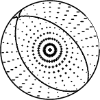
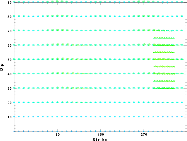
Focal mechanism sensitivity at the preferred depth. The red color indicates a very good fit to thewavefroms.
Each solution is plotted as a vector at a given value of strike and dip with the angle of the vector representing the rake angle, measured, with respect to the upward vertical (N) in the figure.
|
A check on the assumed source location is possible by looking at the time shifts between the observed and predicted traces. The time shifts for waveform matching arise for several reasons:
- The origin time and epicentral distance are incorrect
- The velocity model used for the inversion is incorrect
- The velocity model used to define the P-arrival time is not the
same as the velocity model used for the waveform inversion
(assuming that the initial trace alignment is based on the
P arrival time)
Assuming only a mislocation, the time shifts are fit to a functional form:
Time_shift = A + B cos Azimuth + C Sin Azimuth
The time shifts for this inversion lead to the next figure:
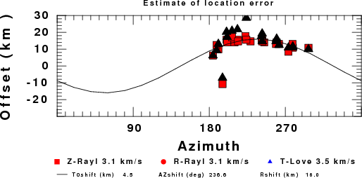
The derived shift in origin time and epicentral coordinates are given at the bottom of the figure.
Discussion
Velocity Model
The nnCIA used for the waveform synthetic seismograms and for the surface wave eigenfunctions and dispersion is as follows:
MODEL.01
C.It. A. Di Luzio et al Earth Plan Lettrs 280 (2009) 1-12 Fig 5. 7-8 MODEL/SURF3
ISOTROPIC
KGS
FLAT EARTH
1-D
CONSTANT VELOCITY
LINE08
LINE09
LINE10
LINE11
      H(KM)   VP(KM/S)   VS(KM/S) RHO(GM/CC)         QP         QS       ETAP       ETAS      FREFP      FREFS
     1.5000     3.7497     2.1436     2.2753  0.500E-02  0.100E-01   0.00       0.00       1.00       1.00
     3.0000     4.9399     2.8210     2.4858  0.500E-02  0.100E-01   0.00       0.00       1.00       1.00
     3.0000     6.0129     3.4336     2.7058  0.500E-02  0.100E-01   0.00       0.00       1.00       1.00
     7.0000     5.5516     3.1475     2.6093  0.167E-02  0.333E-02   0.00       0.00       1.00       1.00
    15.0000     5.8805     3.3583     2.6770  0.167E-02  0.333E-02   0.00       0.00       1.00       1.00
     6.0000     7.1059     4.0081     3.0002  0.167E-02  0.333E-02   0.00       0.00       1.00       1.00
     8.0000     7.1000     3.9864     3.0120  0.167E-02  0.333E-02   0.00       0.00       1.00       1.00
     0.0000     7.9000     4.4036     3.2760  0.167E-02  0.333E-02   0.00       0.00       1.00       1.00
Quality Control
Here we tabulate the reasons for not using certain digital data sets
The following stations did not have a valid response files:
DATE=Thu Aug 22 06:10:29 CDT 2013
Last Changed 2013/08/22