Location
2013/02/16 21:16:09 41.71 13.58 11 4.8 Italy
Arrival Times (from USGS)
Arrival time list
Felt Map
USGS Felt map for this earthquake
USGS Felt reports page for
Focal Mechanism
SLU Moment Tensor Solution
ENS 2013/02/16 21:16:09:0 41.71 13.58 11.0 4.8 Italy
Stations used:
BA.PZUN GE.MATE GU.GORR GU.MAIM GU.POPM IV.ASSB IV.BSSO
IV.CAFR IV.CAMP IV.CERA IV.CERT IV.CESI IV.CESX IV.CING
IV.FAGN IV.FDMO IV.FIAM IV.GIUL IV.GUMA IV.INTR IV.LAV9
IV.LNSS IV.LPEL IV.MELA IV.MGAB IV.MIDA IV.MODR IV.MRLC
IV.MSAG IV.MURB IV.NRCA IV.OFFI IV.PSB1 IV.PTQR IV.PTRJ
IV.RMP IV.RNI2 IV.SACR IV.SACS IV.SAMA IV.SGG IV.SGRT
IV.SNTG IV.TERO IV.TOLF IV.TRIV IV.TRTR IV.VAGA MN.AQU
MN.CUC MN.TIP MN.VLC
Filtering commands used:
hp c 0.02 n 3
lp c 0.06 n 3
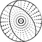
Best Fitting Double Couple
Mo = 1.93e+23 dyne-cm
Mw = 4.79
Z = 17 km
Plane Strike Dip Rake
NP1 317 50 -113
NP2 170 45 -65
Principal Axes:
Axis Value Plunge Azimuth
T 1.93e+23 3 63
N 0.00e+00 17 332
P -1.93e+23 72 161
Moment Tensor: (dyne-cm)
Component Value
Mxx 2.50e+22
Mxy 8.40e+22
Mxz 5.67e+22
Myy 1.50e+23
Myz -1.00e+22
Mzz -1.75e+23
--############
----##################
------######################
######------##################
#######-----------###############
########--------------############ T
########-----------------##########
#########-------------------############
#########--------------------###########
##########----------------------##########
##########-----------------------#########
##########------------------------########
##########----------- ----------########
##########---------- P -----------######
##########---------- -----------######
##########------------------------####
##########-----------------------###
##########----------------------##
#########---------------------
##########------------------
#########-------------
########------
Global CMT Convention Moment Tensor:
R T P
-1.75e+23 5.67e+22 1.00e+22
5.67e+22 2.50e+22 -8.40e+22
1.00e+22 -8.40e+22 1.50e+23
Details of the solution is found at
http://www.eas.slu.edu/eqc/eqc_mt/MECH.IT/20130216211609/index.html
|
Preferred Solution
The preferred solution from an analysis of the surface-wave spectral amplitude radiation pattern, waveform inversion and first motion observations is
      STK = 170
      DIP = 45
     RAKE = -65
       MW = 4.79
       HS = 17.0
The waveform inversion is preferred.
Moment Tensor Comparison
The following compares this source inversion to others
| SLU |
INGVTDMT |
 SLU Moment Tensor Solution
 ENS  2013/02/16 21:16:09:0  41.71   13.58  11.0 4.8 Italy

 Stations used:
   BA.PZUN GE.MATE GU.GORR GU.MAIM GU.POPM IV.ASSB IV.BSSO
   IV.CAFR IV.CAMP IV.CERA IV.CERT IV.CESI IV.CESX IV.CING
   IV.FAGN IV.FDMO IV.FIAM IV.GIUL IV.GUMA IV.INTR IV.LAV9
   IV.LNSS IV.LPEL IV.MELA IV.MGAB IV.MIDA IV.MODR IV.MRLC
   IV.MSAG IV.MURB IV.NRCA IV.OFFI IV.PSB1 IV.PTQR IV.PTRJ
   IV.RMP IV.RNI2 IV.SACR IV.SACS IV.SAMA IV.SGG IV.SGRT
   IV.SNTG IV.TERO IV.TOLF IV.TRIV IV.TRTR IV.VAGA MN.AQU
   MN.CUC MN.TIP MN.VLC

 Filtering commands used:
   hp c 0.02 n 3
   lp c 0.06 n 3

 Best Fitting Double Couple
  Mo = 1.93e+23 dyne-cm
  Mw = 4.79
  Z  = 17 km
  Plane   Strike  Dip  Rake
   NP1      317    50   -113
   NP2      170    45   -65
  Principal Axes:
   Axis    Value   Plunge  Azimuth
    T   1.93e+23      3      63
    N   0.00e+00     17     332
    P  -1.93e+23     72     161

 Moment Tensor: (dyne-cm)
    Component   Value
       Mxx     2.50e+22
       Mxy     8.40e+22
       Mxz     5.67e+22
       Myy     1.50e+23
       Myz    -1.00e+22
       Mzz    -1.75e+23


                     --############
                 ----##################
              ------######################
             ######------##################
           #######-----------###############
          ########--------------############ T
         ########-----------------##########
        #########-------------------############
        #########--------------------###########
       ##########----------------------##########
       ##########-----------------------#########
       ##########------------------------########
       ##########-----------   ----------########
        ##########---------- P -----------######
        ##########----------   -----------######
         ##########------------------------####
          ##########-----------------------###
           ##########----------------------##
             #########---------------------
              ##########------------------
                 #########-------------
                     ########------


 Global CMT Convention Moment Tensor:
      R          T          P
 -1.75e+23   5.67e+22   1.00e+22
  5.67e+22   2.50e+22  -8.40e+22
  1.00e+22  -8.40e+22   1.50e+23


Details of the solution is found at

http://www.eas.slu.edu/eqc/eqc_mt/MECH.IT/20130216211609/index.html
|
|
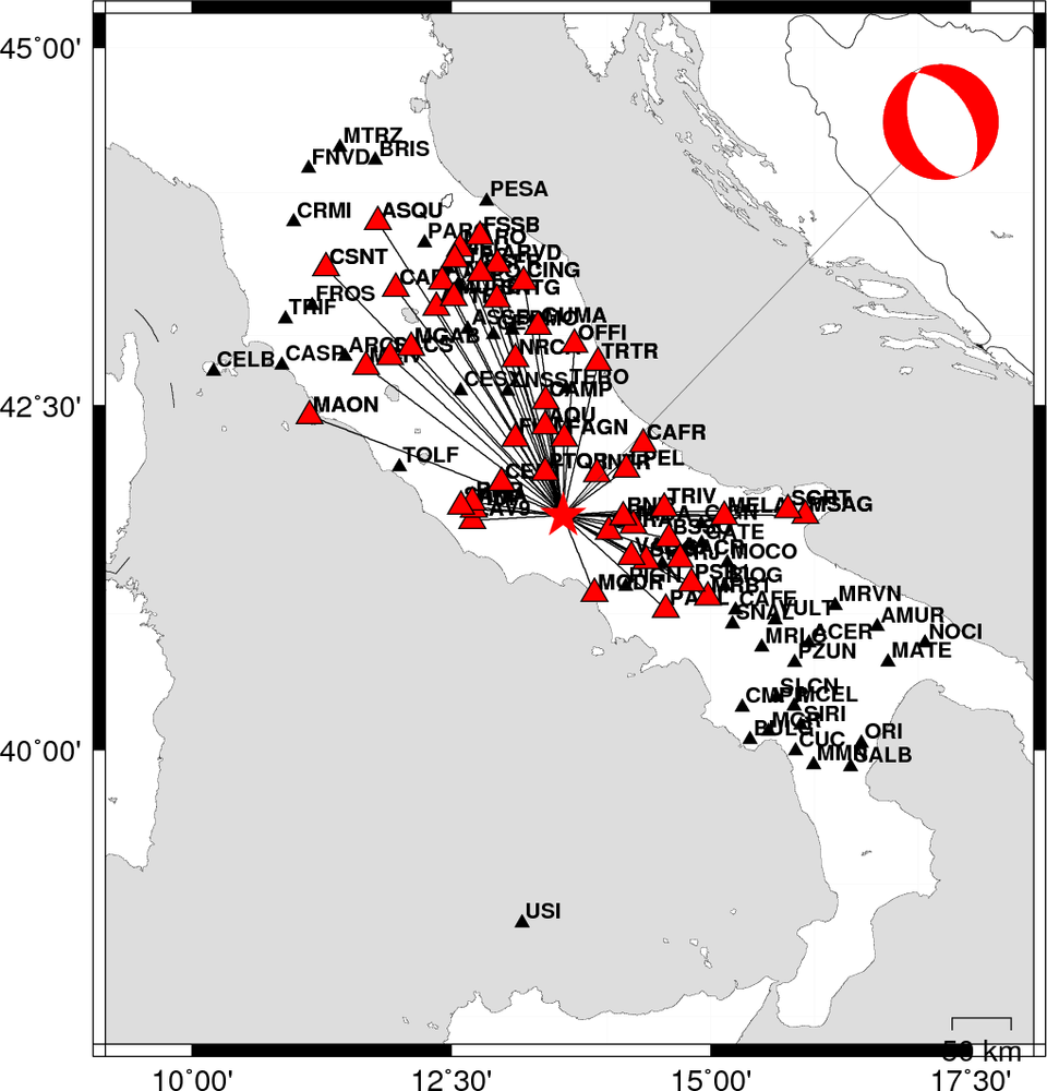
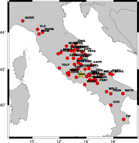
Waveform Inversion
The focal mechanism was determined using broadband seismic waveforms. The location of the event and the
and stations used for the waveform inversion are shown in the next figure.
|
|
Location of broadband stations used for waveform inversion
|
The program wvfgrd96 was used with good traces observed at short distance to determine the focal mechanism, depth and seismic moment. This technique requires a high quality signal and well determined velocity model for the Green functions. To the extent that these are the quality data, this type of mechanism should be preferred over the radiation pattern technique which requires the separate step of defining the pressure and tension quadrants and the correct strike.
The observed and predicted traces are filtered using the following gsac commands:
hp c 0.02 n 3
lp c 0.06 n 3
The results of this grid search from 0.5 to 19 km depth are as follow:
           DEPTH  STK   DIP  RAKE   MW    FIT
WVFGRD96    1.0    60    50    90   4.51 0.3554
WVFGRD96    2.0   245    45    95   4.57 0.3586
WVFGRD96    3.0    30    70    55   4.60 0.3436
WVFGRD96    4.0    25    80    45   4.59 0.3581
WVFGRD96    5.0   200    90   -55   4.66 0.3798
WVFGRD96    6.0    20    90    50   4.66 0.4058
WVFGRD96    7.0   190    75   -50   4.67 0.4334
WVFGRD96    8.0   180    60   -55   4.68 0.4717
WVFGRD96    9.0   170    45   -65   4.72 0.5146
WVFGRD96   10.0   170    45   -65   4.73 0.5522
WVFGRD96   11.0   170    45   -65   4.74 0.5807
WVFGRD96   12.0   170    45   -65   4.74 0.6022
WVFGRD96   13.0   170    45   -65   4.75 0.6185
WVFGRD96   14.0   170    45   -65   4.76 0.6309
WVFGRD96   15.0   170    45   -65   4.78 0.6423
WVFGRD96   16.0   170    45   -65   4.79 0.6485
WVFGRD96   17.0   170    45   -65   4.79 0.6508
WVFGRD96   18.0   170    45   -65   4.80 0.6499
WVFGRD96   19.0   170    45   -65   4.80 0.6462
WVFGRD96   20.0   170    45   -65   4.80 0.6401
WVFGRD96   21.0   175    45   -60   4.81 0.6320
WVFGRD96   22.0   175    50   -55   4.81 0.6223
WVFGRD96   23.0   175    50   -55   4.82 0.6120
WVFGRD96   24.0   175    50   -55   4.82 0.5995
WVFGRD96   25.0   175    50   -55   4.83 0.5853
WVFGRD96   26.0   175    55   -60   4.83 0.5721
WVFGRD96   27.0   170    55   -65   4.84 0.5582
WVFGRD96   28.0   170    55   -65   4.85 0.5442
WVFGRD96   29.0   170    55   -65   4.86 0.5290
The best solution is
WVFGRD96 17.0 170 45 -65 4.79 0.6508
The mechanism correspond to the best fit is
|
|
Figure 1. Waveform inversion focal mechanism
|
The best fit as a function of depth is given in the following figure:
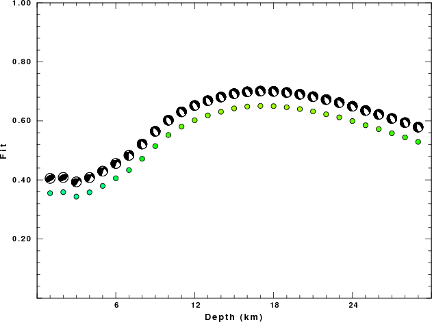
|
|
Figure 2. Depth sensitivity for waveform mechanism
|
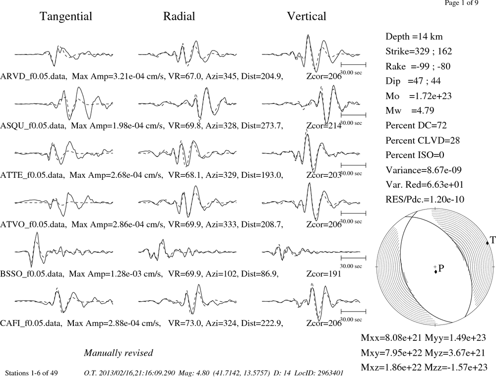
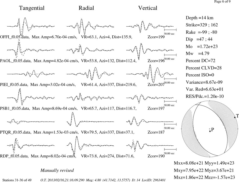
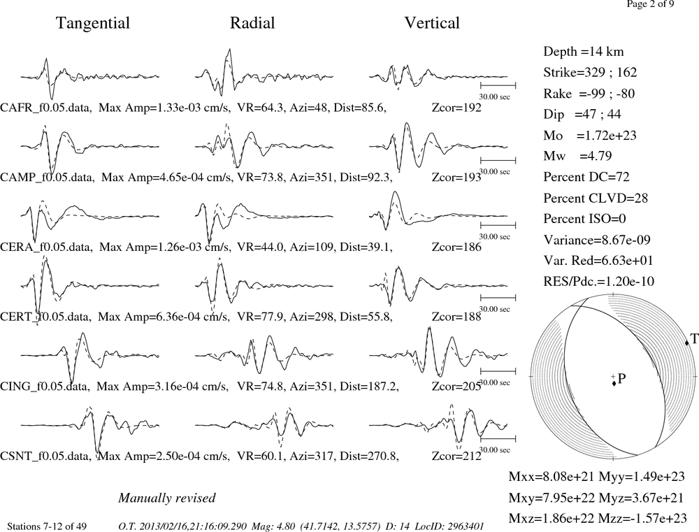
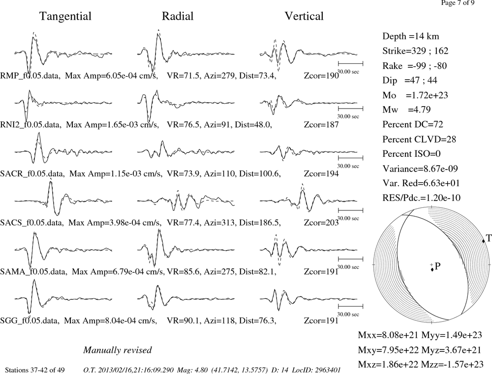
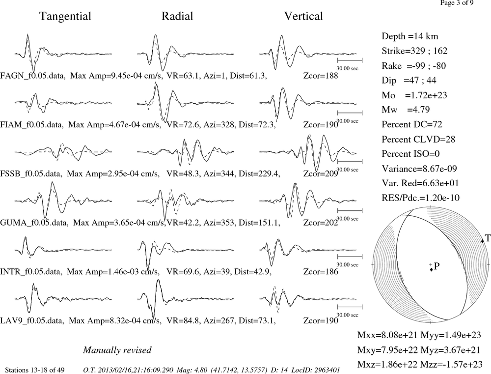
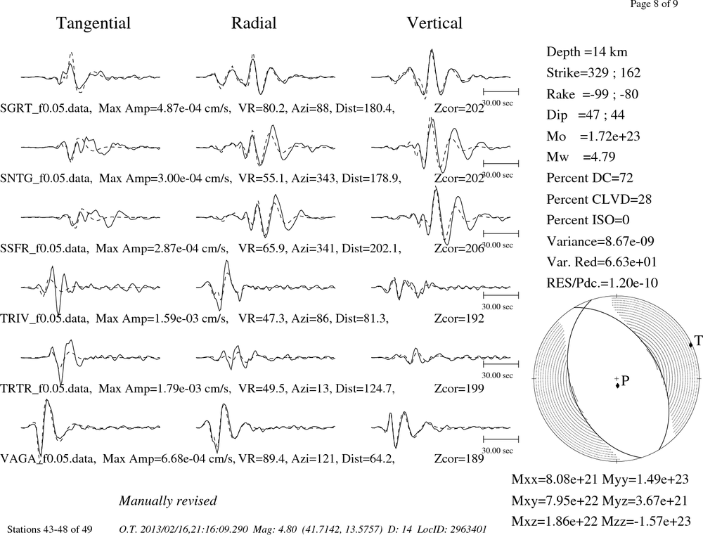
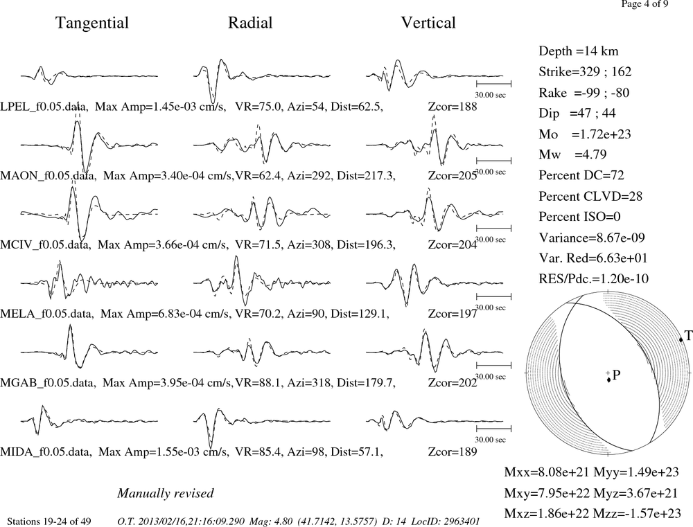
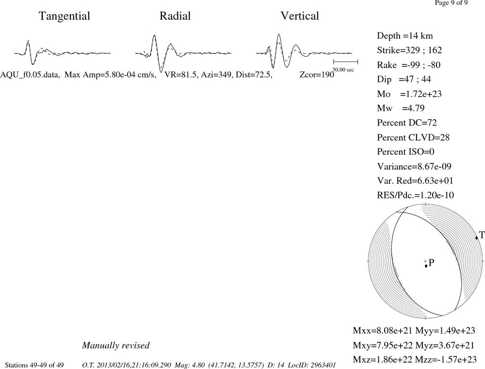
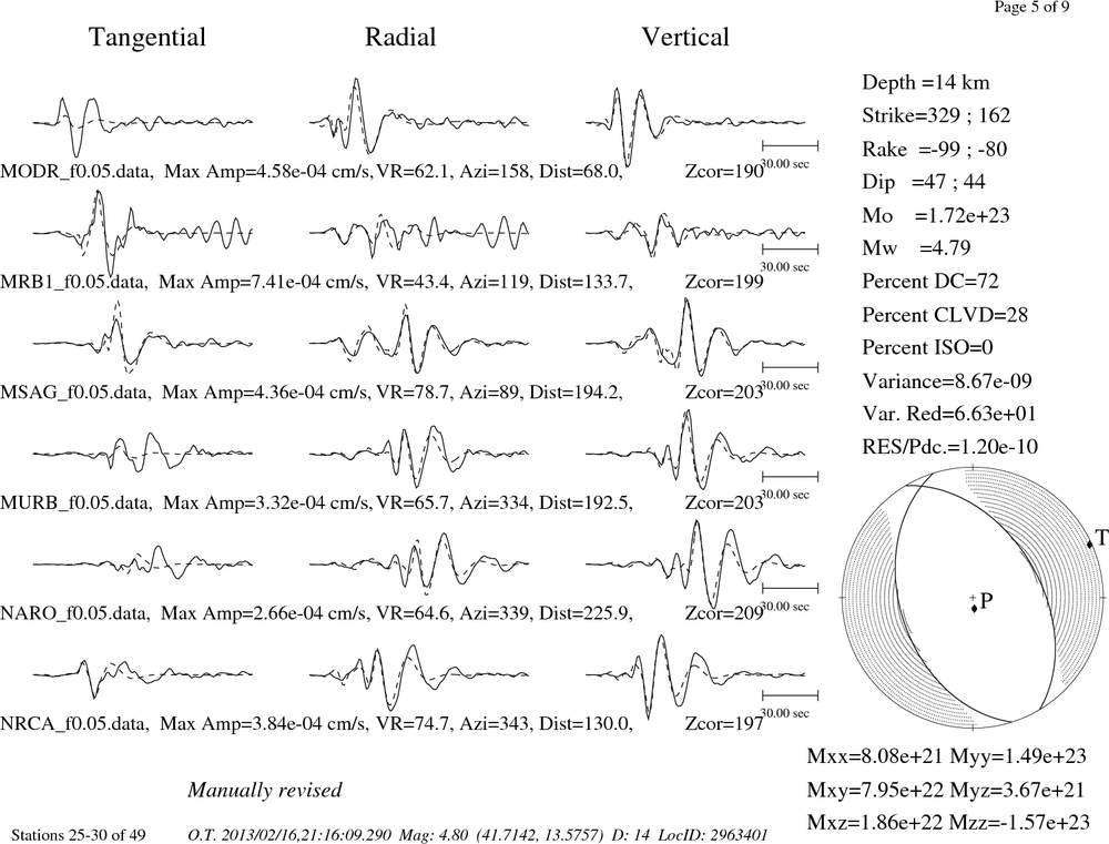
The comparison of the observed and predicted waveforms is given in the next figure. The red traces are the observed and the blue are the predicted.
Each observed-predicted component is plotted to the same scale and peak amplitudes are indicated by the numbers to the left of each trace. A pair of numbers is given in black at the right of each predicted traces. The upper number it the time shift required for maximum correlation between the observed and predicted traces. This time shift is required because the synthetics are not computed at exactly the same distance as the observed and because the velocity model used in the predictions may not be perfect.
A positive time shift indicates that the prediction is too fast and should be delayed to match the observed trace (shift to the right in this figure). A negative value indicates that the prediction is too slow. The lower number gives the percentage of variance reduction to characterize the individual goodness of fit (100% indicates a perfect fit).
The bandpass filter used in the processing and for the display was
hp c 0.02 n 3
lp c 0.06 n 3
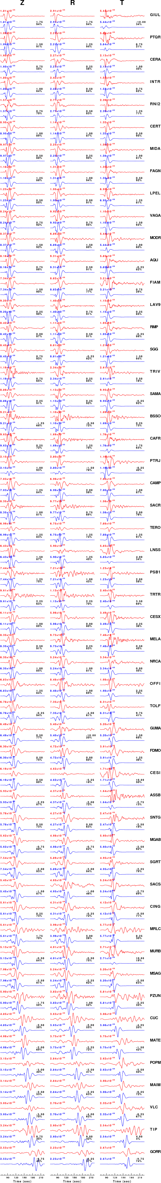
|
|
Figure 3. Waveform comparison for selected depth
|
|
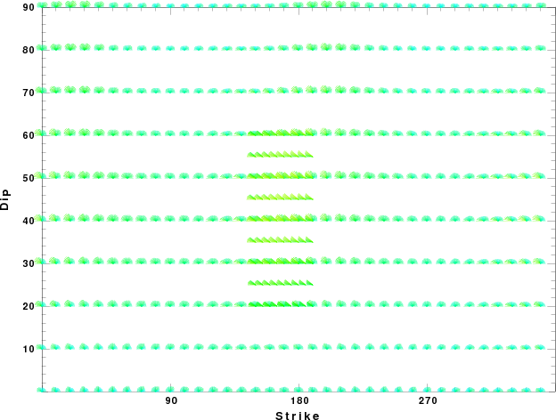
|
Focal mechanism sensitivity at the preferred depth. The red color indicates a very good fit to thewavefroms.
Each solution is plotted as a vector at a given value of strike and dip with the angle of the vector representing the rake angle, measured, with respect to the upward vertical (N) in the figure.
|
A check on the assumed source location is possible by looking at the time shifts between the observed and predicted traces. The time shifts for waveform matching arise for several reasons:
- The origin time and epicentral distance are incorrect
- The velocity model used for the inversion is incorrect
- The velocity model used to define the P-arrival time is not the
same as the velocity model used for the waveform inversion
(assuming that the initial trace alignment is based on the
P arrival time)
Assuming only a mislocation, the time shifts are fit to a functional form:
Time_shift = A + B cos Azimuth + C Sin Azimuth
The time shifts for this inversion lead to the next figure:
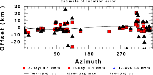
The derived shift in origin time and epicentral coordinates are given at the bottom of the figure.
Discussion
Velocity Model
The nnCIA used for the waveform synthetic seismograms and for the surface wave eigenfunctions and dispersion is as follows:
MODEL.01
C.It. A. Di Luzio et al Earth Plan Lettrs 280 (2009) 1-12 Fig 5. 7-8 MODEL/SURF3
ISOTROPIC
KGS
FLAT EARTH
1-D
CONSTANT VELOCITY
LINE08
LINE09
LINE10
LINE11
      H(KM)   VP(KM/S)   VS(KM/S) RHO(GM/CC)         QP         QS       ETAP       ETAS      FREFP      FREFS
     1.5000     3.7497     2.1436     2.2753  0.500E-02  0.100E-01   0.00       0.00       1.00       1.00
     3.0000     4.9399     2.8210     2.4858  0.500E-02  0.100E-01   0.00       0.00       1.00       1.00
     3.0000     6.0129     3.4336     2.7058  0.500E-02  0.100E-01   0.00       0.00       1.00       1.00
     7.0000     5.5516     3.1475     2.6093  0.167E-02  0.333E-02   0.00       0.00       1.00       1.00
    15.0000     5.8805     3.3583     2.6770  0.167E-02  0.333E-02   0.00       0.00       1.00       1.00
     6.0000     7.1059     4.0081     3.0002  0.167E-02  0.333E-02   0.00       0.00       1.00       1.00
     8.0000     7.1000     3.9864     3.0120  0.167E-02  0.333E-02   0.00       0.00       1.00       1.00
     0.0000     7.9000     4.4036     3.2760  0.167E-02  0.333E-02   0.00       0.00       1.00       1.00
Quality Control
Here we tabulate the reasons for not using certain digital data sets
The following stations did not have a valid response files:
DATE=Mon Feb 18 07:16:33 CST 2013
Last Changed 2013/02/16