Location
2013/01/25 14:48:18 44.168 10.454 15.5 4.8 Italy
Arrival Times (from USGS)
Arrival time list
Felt Map
USGS Felt map for this earthquake
USGS Felt reports page for
Focal Mechanism
 SLU Moment Tensor Solution
 ENS  2013/01/25 14:48:18:0  44.17   10.45  15.5 4.8 Italy

 Stations used:
   CH.AIGLE CH.BERGE CH.BERNI CH.BNALP CH.BOURR CH.BRANT
   CH.DAVOX CH.DIX CH.EMBD CH.FIESA CH.FUORN CH.FUSIO CH.HASLI
   CH.LAUCH CH.LIENZ CH.LLS CH.MMK CH.MUGIO CH.MUO CH.OTER1
   CH.PANIX CH.PLONS CH.SENIN CH.SLE CH.SULZ CH.VDL CH.WILA
   CH.ZUR FR.ARBF FR.ARTF FR.CALF FR.EILF FR.ESCA FR.ISO
   FR.MON FR.OG35 FR.OGAG FR.OGDI FR.SAOF FR.SURF GU.BHB
   GU.ENR GU.EQUI GU.FINB GU.MAIM GU.NEGI GU.PCP GU.PZZ
   GU.REMY GU.RORO GU.RRL GU.RSP GU.SATI GU.STV GU.TRAV IV.AOI
   IV.ARCI IV.ARVD IV.BRMO IV.CAFI IV.CAFR IV.CAMP IV.CASP
   IV.CELB IV.CESX IV.CING IV.CRE IV.CSNT IV.FAGN IV.FDMO
   IV.FSSB IV.FVI IV.GUMA IV.INTR IV.LATE IV.LPEL IV.MAON
   IV.MGAB IV.MTCE IV.MURB IV.NRCA IV.PESA IV.PIEI IV.PTCC
   IV.PTQR IV.SNTG IV.SSFR IV.STAL IV.TERO IV.TRTR IV.ZCCA
   MN.AQU MN.TUE OE.OBKA

 Filtering commands used:
   hp c 0.02 n 3
   lp c 0.05 n 3

 Best Fitting Double Couple
  Mo = 1.62e+23 dyne-cm
  Mw = 4.74
  Z  = 16 km
  Plane   Strike  Dip  Rake
   NP1       56    76   164
   NP2      150    75    15
  Principal Axes:
   Axis    Value   Plunge  Azimuth
    T   1.62e+23     21      13
    N   0.00e+00     69     194
    P  -1.62e+23      0     103

 Moment Tensor: (dyne-cm)
    Component   Value
       Mxx     1.26e+23
       Mxy     6.66e+22
       Mxz     5.33e+22
       Myy    -1.47e+23
       Myz     1.12e+22
       Mzz     2.10e+22


                     ##############
                 -############   ######
              ----############ T #########
             -----############   ##########
           --------##########################
          ---------#########################--
         -----------#######################----
        -------------####################-------
        -------------###################--------
       ---------------################-----------
       ----------------############--------------
       -----------------#########----------------
       ------------------######---------------
        ------------------##------------------ P
        -----------------###------------------
         ------------########------------------
          -------#############----------------
           #####################-------------
             ####################----------
              #####################-------
                 #####################-
                     ##############


 Global CMT Convention Moment Tensor:
      R          T          P
  2.10e+22   5.33e+22  -1.12e+22
  5.33e+22   1.26e+23  -6.66e+22
 -1.12e+22  -6.66e+22  -1.47e+23


Details of the solution is found at

http://www.eas.slu.edu/eqc/eqc_mt/MECH.IT/20130125144818/index.html
|
Preferred Solution
The preferred solution from an analysis of the surface-wave spectral amplitude radiation pattern, waveform inversion and first motion observations is
      STK = 150
      DIP = 75
     RAKE = 15
       MW = 4.74
       HS = 16.0
The waveform inversion is preferred.
Moment Tensor Comparison
The following compares this source inversion to others
| SLU |
INGVTDMT |
 SLU Moment Tensor Solution
 ENS  2013/01/25 14:48:18:0  44.17   10.45  15.5 4.8 Italy

 Stations used:
   CH.AIGLE CH.BERGE CH.BERNI CH.BNALP CH.BOURR CH.BRANT
   CH.DAVOX CH.DIX CH.EMBD CH.FIESA CH.FUORN CH.FUSIO CH.HASLI
   CH.LAUCH CH.LIENZ CH.LLS CH.MMK CH.MUGIO CH.MUO CH.OTER1
   CH.PANIX CH.PLONS CH.SENIN CH.SLE CH.SULZ CH.VDL CH.WILA
   CH.ZUR FR.ARBF FR.ARTF FR.CALF FR.EILF FR.ESCA FR.ISO
   FR.MON FR.OG35 FR.OGAG FR.OGDI FR.SAOF FR.SURF GU.BHB
   GU.ENR GU.EQUI GU.FINB GU.MAIM GU.NEGI GU.PCP GU.PZZ
   GU.REMY GU.RORO GU.RRL GU.RSP GU.SATI GU.STV GU.TRAV IV.AOI
   IV.ARCI IV.ARVD IV.BRMO IV.CAFI IV.CAFR IV.CAMP IV.CASP
   IV.CELB IV.CESX IV.CING IV.CRE IV.CSNT IV.FAGN IV.FDMO
   IV.FSSB IV.FVI IV.GUMA IV.INTR IV.LATE IV.LPEL IV.MAON
   IV.MGAB IV.MTCE IV.MURB IV.NRCA IV.PESA IV.PIEI IV.PTCC
   IV.PTQR IV.SNTG IV.SSFR IV.STAL IV.TERO IV.TRTR IV.ZCCA
   MN.AQU MN.TUE OE.OBKA

 Filtering commands used:
   hp c 0.02 n 3
   lp c 0.05 n 3

 Best Fitting Double Couple
  Mo = 1.62e+23 dyne-cm
  Mw = 4.74
  Z  = 16 km
  Plane   Strike  Dip  Rake
   NP1       56    76   164
   NP2      150    75    15
  Principal Axes:
   Axis    Value   Plunge  Azimuth
    T   1.62e+23     21      13
    N   0.00e+00     69     194
    P  -1.62e+23      0     103

 Moment Tensor: (dyne-cm)
    Component   Value
       Mxx     1.26e+23
       Mxy     6.66e+22
       Mxz     5.33e+22
       Myy    -1.47e+23
       Myz     1.12e+22
       Mzz     2.10e+22


                     ##############
                 -############   ######
              ----############ T #########
             -----############   ##########
           --------##########################
          ---------#########################--
         -----------#######################----
        -------------####################-------
        -------------###################--------
       ---------------################-----------
       ----------------############--------------
       -----------------#########----------------
       ------------------######---------------
        ------------------##------------------ P
        -----------------###------------------
         ------------########------------------
          -------#############----------------
           #####################-------------
             ####################----------
              #####################-------
                 #####################-
                     ##############


 Global CMT Convention Moment Tensor:
      R          T          P
  2.10e+22   5.33e+22  -1.12e+22
  5.33e+22   1.26e+23  -6.66e+22
 -1.12e+22  -6.66e+22  -1.47e+23


Details of the solution is found at

http://www.eas.slu.edu/eqc/eqc_mt/MECH.IT/20130125144818/index.html
|
|
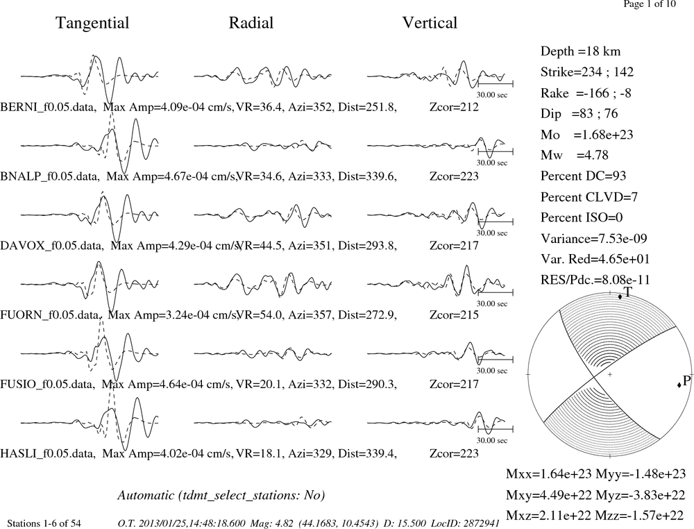
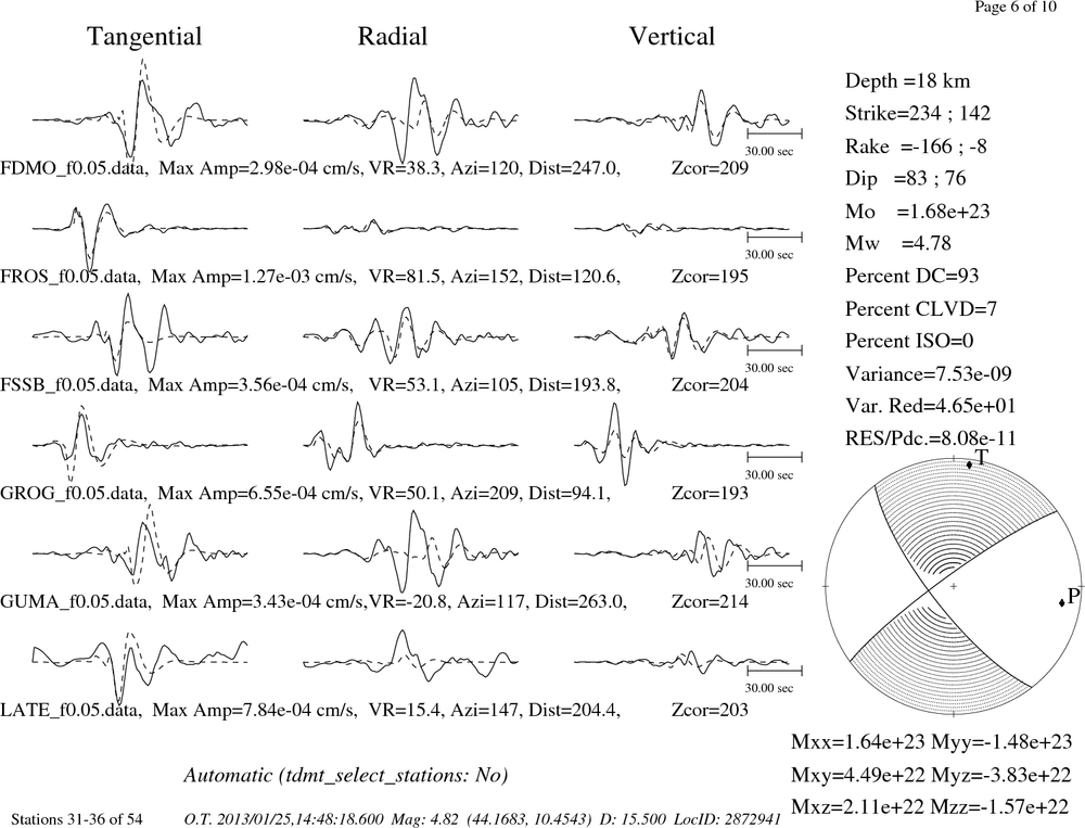
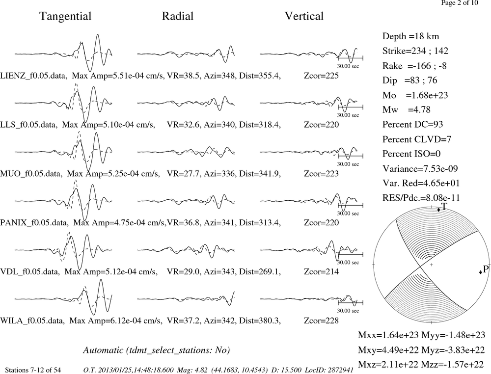
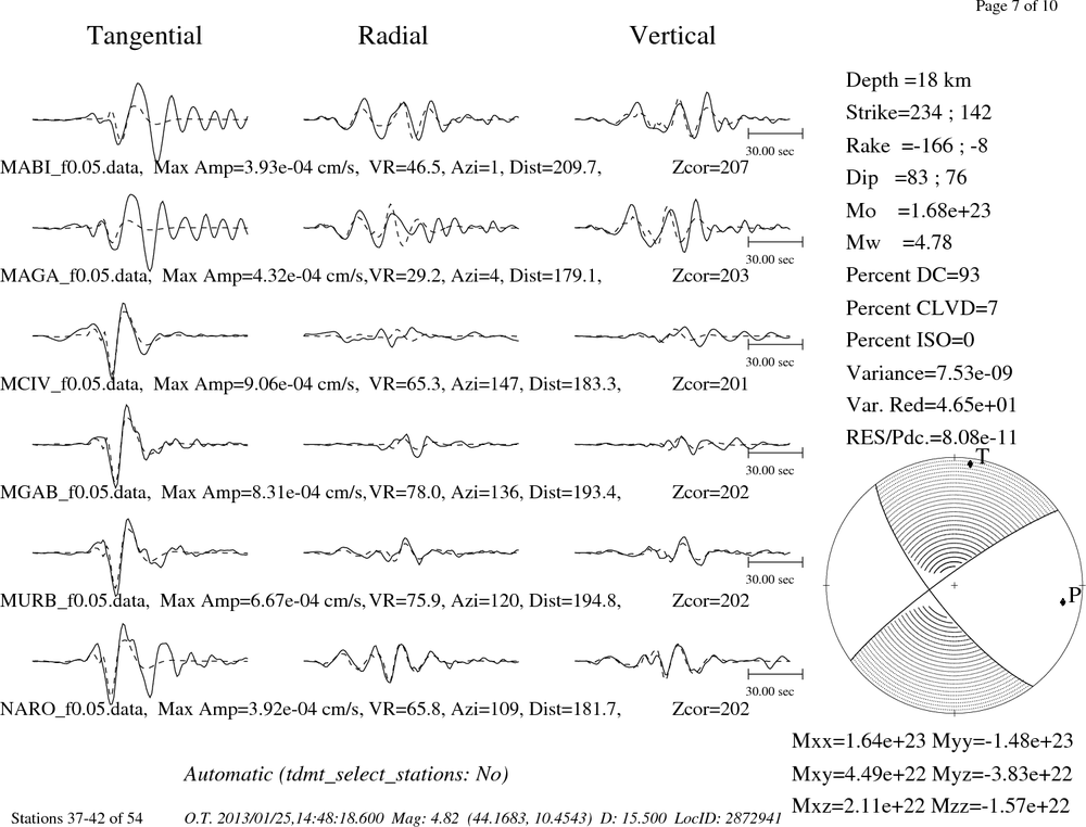
Waveform Inversion
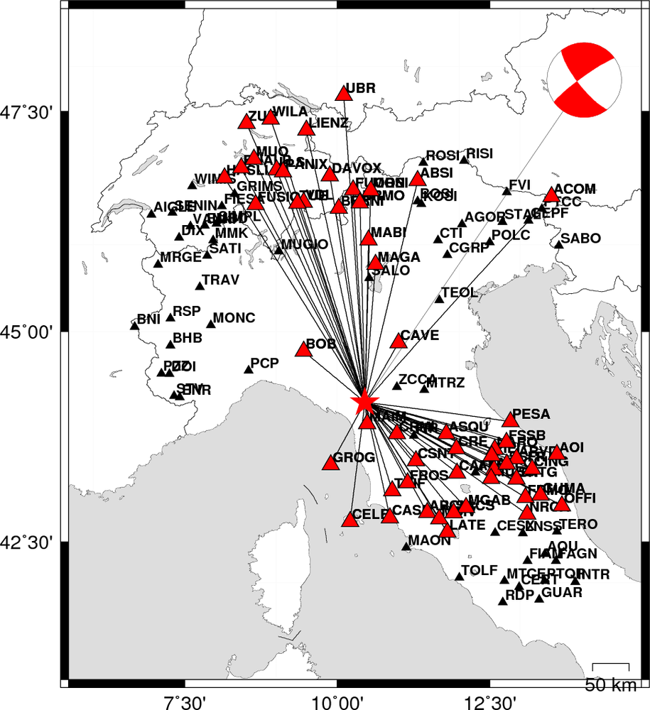
The focal mechanism was determined using broadband seismic waveforms. The location of the event and the
and stations used for the waveform inversion are shown in the next figure.
|
|
Location of broadband stations used for waveform inversion
|
The program wvfgrd96 was used with good traces observed at short distance to determine the focal mechanism, depth and seismic moment. This technique requires a high quality signal and well determined velocity model for the Green functions. To the extent that these are the quality data, this type of mechanism should be preferred over the radiation pattern technique which requires the separate step of defining the pressure and tension quadrants and the correct strike.
The observed and predicted traces are filtered using the following gsac commands:
hp c 0.02 n 3
lp c 0.05 n 3
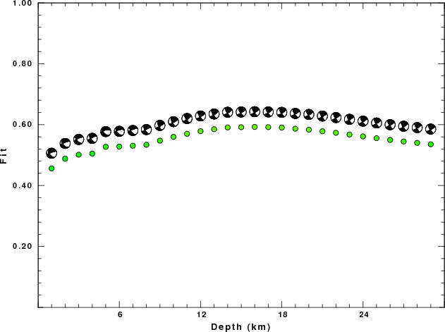
The results of this grid search from 0.5 to 19 km depth are as follow:
           DEPTH  STK   DIP  RAKE   MW    FIT
WVFGRD96    1.0   145    50   -20   4.59 0.4562
WVFGRD96    2.0   140    50   -25   4.62 0.4883
WVFGRD96    3.0   140    55   -25   4.62 0.5014
WVFGRD96    4.0   145    65   -15   4.60 0.5050
WVFGRD96    5.0   135    50   -40   4.69 0.5272
WVFGRD96    6.0   140    50   -35   4.69 0.5281
WVFGRD96    7.0   145    55   -25   4.67 0.5307
WVFGRD96    8.0   150    65    -5   4.64 0.5338
WVFGRD96    9.0   155    65    15   4.66 0.5474
WVFGRD96   10.0   155    65    15   4.67 0.5598
WVFGRD96   11.0   150    70    15   4.68 0.5701
WVFGRD96   12.0   150    70    15   4.69 0.5786
WVFGRD96   13.0   150    70    15   4.70 0.5850
WVFGRD96   14.0   150    75    15   4.72 0.5907
WVFGRD96   15.0   150    70    15   4.73 0.5916
WVFGRD96   16.0   150    75    15   4.74 0.5925
WVFGRD96   17.0   150    75    15   4.75 0.5918
WVFGRD96   18.0   150    75    15   4.76 0.5903
WVFGRD96   19.0   150    75    10   4.77 0.5868
WVFGRD96   20.0   150    75    10   4.78 0.5834
WVFGRD96   21.0   150    75    10   4.78 0.5782
WVFGRD96   22.0   150    75    10   4.79 0.5733
WVFGRD96   23.0   150    75    10   4.80 0.5675
WVFGRD96   24.0   150    75    10   4.82 0.5614
WVFGRD96   25.0   150    75    10   4.83 0.5555
WVFGRD96   26.0   150    75    10   4.84 0.5498
WVFGRD96   27.0   150    75    10   4.85 0.5448
WVFGRD96   28.0   150    75    10   4.87 0.5402
WVFGRD96   29.0   150    75    10   4.88 0.5355
The best solution is
WVFGRD96 16.0 150 75 15 4.74 0.5925
The mechanism correspond to the best fit is
|
|
Figure 1. Waveform inversion focal mechanism
|
The best fit as a function of depth is given in the following figure:
|
|
Figure 2. Depth sensitivity for waveform mechanism
|
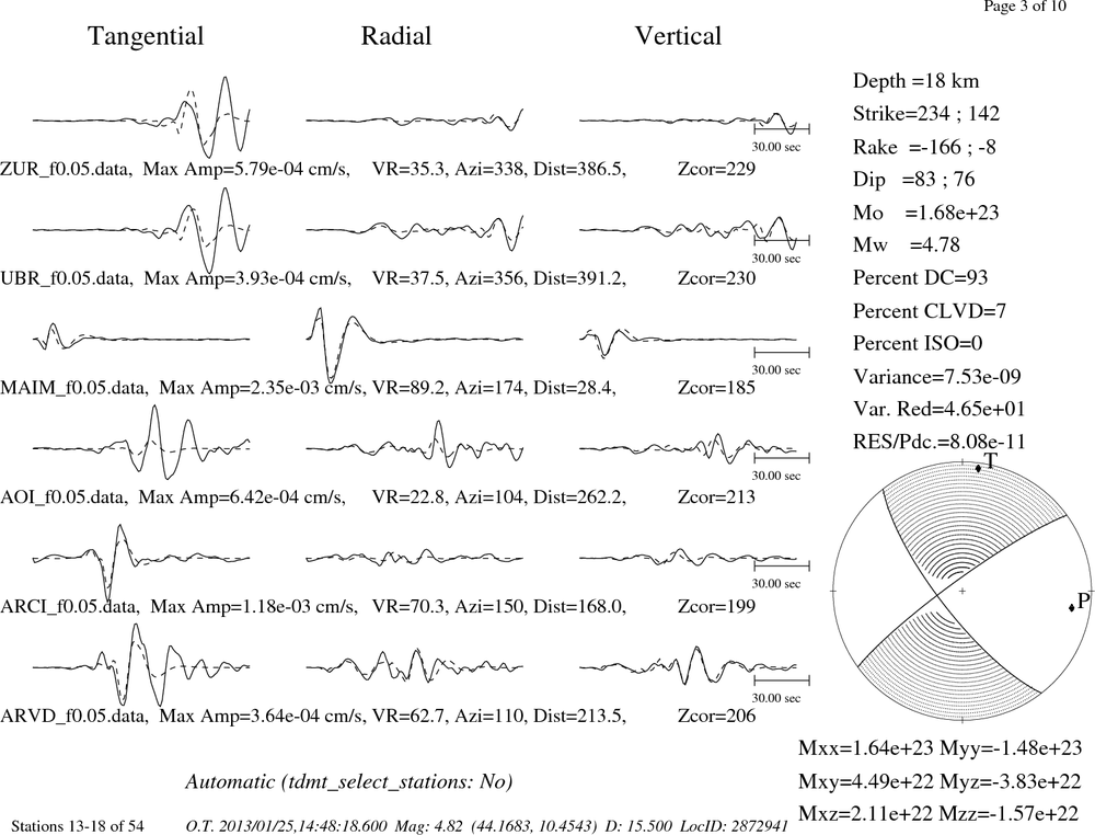
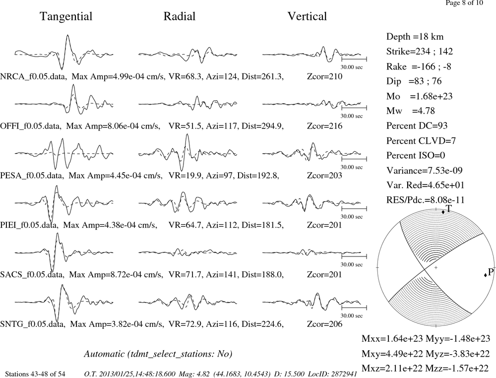
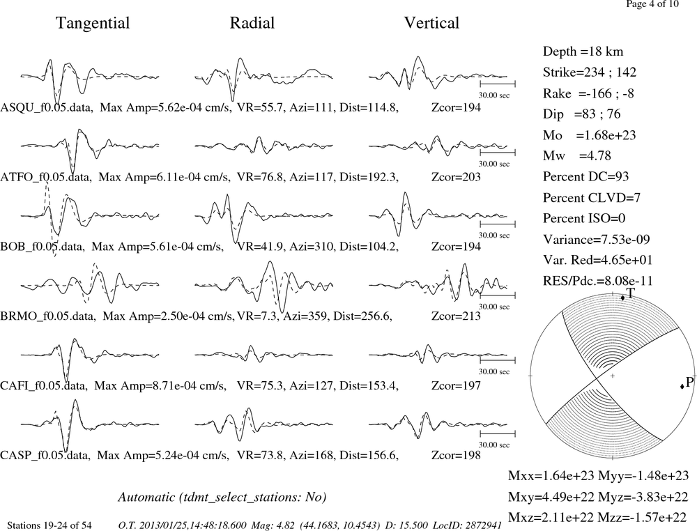
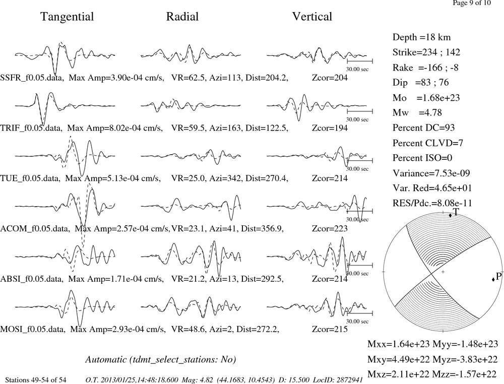
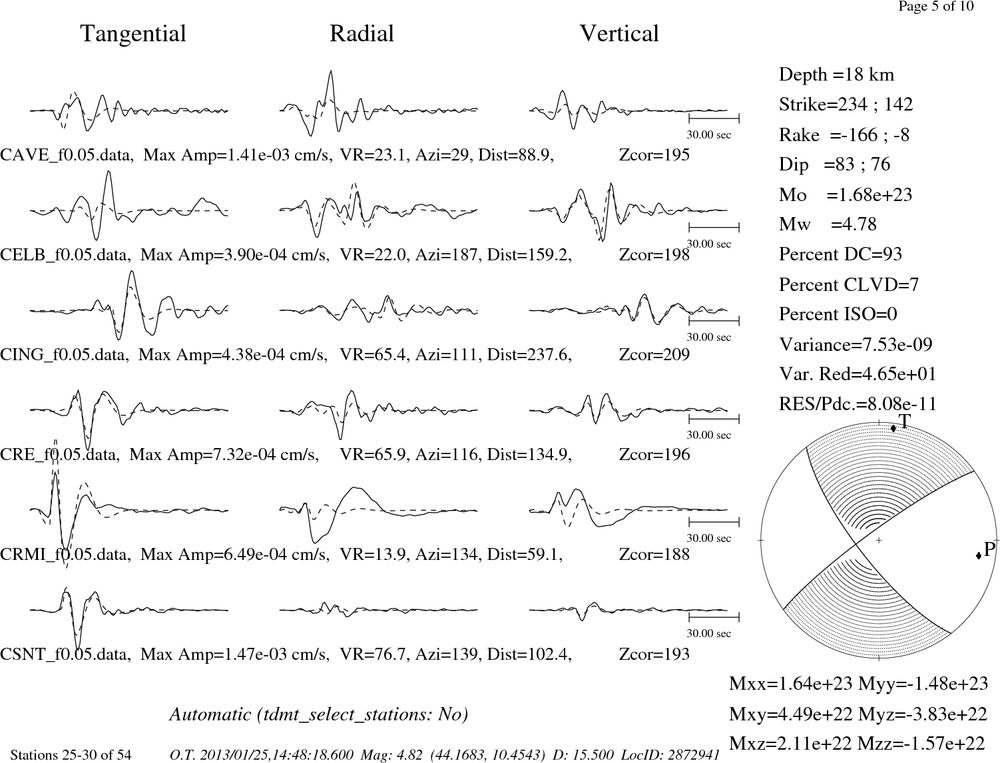
The comparison of the observed and predicted waveforms is given in the next figure. The red traces are the observed and the blue are the predicted.
Each observed-predicted component is plotted to the same scale and peak amplitudes are indicated by the numbers to the left of each trace. A pair of numbers is given in black at the right of each predicted traces. The upper number it the time shift required for maximum correlation between the observed and predicted traces. This time shift is required because the synthetics are not computed at exactly the same distance as the observed and because the velocity model used in the predictions may not be perfect.
A positive time shift indicates that the prediction is too fast and should be delayed to match the observed trace (shift to the right in this figure). A negative value indicates that the prediction is too slow. The lower number gives the percentage of variance reduction to characterize the individual goodness of fit (100% indicates a perfect fit).
The bandpass filter used in the processing and for the display was
hp c 0.02 n 3
lp c 0.05 n 3

|
|
Figure 3. Waveform comparison for selected depth
|
|
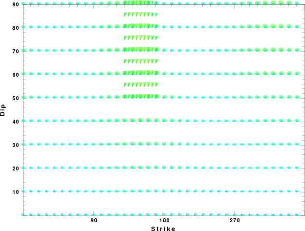
|
Focal mechanism sensitivity at the preferred depth. The red color indicates a very good fit to thewavefroms.
Each solution is plotted as a vector at a given value of strike and dip with the angle of the vector representing the rake angle, measured, with respect to the upward vertical (N) in the figure.
|
A check on the assumed source location is possible by looking at the time shifts between the observed and predicted traces. The time shifts for waveform matching arise for several reasons:
- The origin time and epicentral distance are incorrect
- The velocity model used for the inversion is incorrect
- The velocity model used to define the P-arrival time is not the
same as the velocity model used for the waveform inversion
(assuming that the initial trace alignment is based on the
P arrival time)
Assuming only a mislocation, the time shifts are fit to a functional form:
Time_shift = A + B cos Azimuth + C Sin Azimuth
The time shifts for this inversion lead to the next figure:
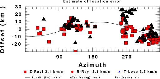
The derived shift in origin time and epicentral coordinates are given at the bottom of the figure.
Discussion
Velocity Model
The nnCIA used for the waveform synthetic seismograms and for the surface wave eigenfunctions and dispersion is as follows:
MODEL.01
C.It. A. Di Luzio et al Earth Plan Lettrs 280 (2009) 1-12 Fig 5. 7-8 MODEL/SURF3
ISOTROPIC
KGS
FLAT EARTH
1-D
CONSTANT VELOCITY
LINE08
LINE09
LINE10
LINE11
      H(KM)   VP(KM/S)   VS(KM/S) RHO(GM/CC)         QP         QS       ETAP       ETAS      FREFP      FREFS
     1.5000     3.7497     2.1436     2.2753  0.500E-02  0.100E-01   0.00       0.00       1.00       1.00
     3.0000     4.9399     2.8210     2.4858  0.500E-02  0.100E-01   0.00       0.00       1.00       1.00
     3.0000     6.0129     3.4336     2.7058  0.500E-02  0.100E-01   0.00       0.00       1.00       1.00
     7.0000     5.5516     3.1475     2.6093  0.167E-02  0.333E-02   0.00       0.00       1.00       1.00
    15.0000     5.8805     3.3583     2.6770  0.167E-02  0.333E-02   0.00       0.00       1.00       1.00
     6.0000     7.1059     4.0081     3.0002  0.167E-02  0.333E-02   0.00       0.00       1.00       1.00
     8.0000     7.1000     3.9864     3.0120  0.167E-02  0.333E-02   0.00       0.00       1.00       1.00
     0.0000     7.9000     4.4036     3.2760  0.167E-02  0.333E-02   0.00       0.00       1.00       1.00
Quality Control
Here we tabulate the reasons for not using certain digital data sets
The following stations did not have a valid response files:
DATE=Sat Jan 26 08:05:42 CST 2013
Last Changed 2013/01/25