Location

2013/01/04 07:50:06 37.873 14.722 10.1 4.3 Italy

Arrival Times (from USGS)

Arrival time list

Felt Map

USGS Felt map for this earthquake

USGS Felt reports page for

Focal Mechanism

SLU Moment Tensor Solution ENS 2013/01/04 07:50:06:0 37.87 14.72 10.1 4.3 Italy Stations used: IV.ALJA IV.GALF IV.GIB IV.HAGA IV.HAVL IV.HCRL IV.HMDC IV.MILZ IV.MPAZ IV.MSCL IV.MSFR IV.MSRU IV.NOV IV.SOLUN MN.CEL Filtering commands used: hp c 0.02 n 3 lp c 0.06 n 3 Best Fitting Double Couple Mo = 1.60e+22 dyne-cm Mw = 4.07 Z = 9 km Plane Strike Dip Rake NP1 88 56 -113 NP2 305 40 -60 Principal Axes: Axis Value Plunge Azimuth T 1.60e+22 9 194 N 0.00e+00 19 101 P -1.60e+22 69 307 Moment Tensor: (dyne-cm) Component Value Mxx 1.40e+22 Mxy 4.66e+21 Mxz -5.50e+21 Myy -3.44e+20 Myz 3.65e+21 Mzz -1.37e+22 ############## ###################### ############################ ##------------################ ---------------------############# -------------------------########### ----------------------------########## -------------------------------######### --------------- ---------------####### ---------------- P ----------------####### ---------------- -----------------###### -------------------------------------###-- ##---------------------------------------- ####-------------------------------##--- #######------------------------######--- ##############--------##############-- ###################################- ################################## ############################## ############################ ##### ############## # T ########## Global CMT Convention Moment Tensor: R T P -1.37e+22 -5.50e+21 -3.65e+21 -5.50e+21 1.40e+22 -4.66e+21 -3.65e+21 -4.66e+21 -3.44e+20 Details of the solution is found at http://www.eas.slu.edu/eqc/eqc_mt/MECH.IT/20130104075006/index.html

Preferred Solution

      STK = 305
      DIP = 40
     RAKE = -60
       MW = 4.07
       HS = 9.0

The waveform inversion is preferred.

Moment Tensor Comparison

The following compares this source inversion to others

SLU

INGVTDMT

SLU Moment Tensor Solution ENS 2013/01/04 07:50:06:0 37.87 14.72 10.1 4.3 Italy Stations used: IV.ALJA IV.GALF IV.GIB IV.HAGA IV.HAVL IV.HCRL IV.HMDC IV.MILZ IV.MPAZ IV.MSCL IV.MSFR IV.MSRU IV.NOV IV.SOLUN MN.CEL Filtering commands used: hp c 0.02 n 3 lp c 0.06 n 3 Best Fitting Double Couple Mo = 1.60e+22 dyne-cm Mw = 4.07 Z = 9 km Plane Strike Dip Rake NP1 88 56 -113 NP2 305 40 -60 Principal Axes: Axis Value Plunge Azimuth T 1.60e+22 9 194 N 0.00e+00 19 101 P -1.60e+22 69 307 Moment Tensor: (dyne-cm) Component Value Mxx 1.40e+22 Mxy 4.66e+21 Mxz -5.50e+21 Myy -3.44e+20 Myz 3.65e+21 Mzz -1.37e+22 ############## ###################### ############################ ##------------################ ---------------------############# -------------------------########### ----------------------------########## -------------------------------######### --------------- ---------------####### ---------------- P ----------------####### ---------------- -----------------###### -------------------------------------###-- ##---------------------------------------- ####-------------------------------##--- #######------------------------######--- ##############--------##############-- ###################################- ################################## ############################## ############################ ##### ############## # T ########## Global CMT Convention Moment Tensor: R T P -1.37e+22 -5.50e+21 -3.65e+21 -5.50e+21 1.40e+22 -4.66e+21 -3.65e+21 -4.66e+21 -3.44e+20 Details of the solution is found at http://www.eas.slu.edu/eqc/eqc_mt/MECH.IT/20130104075006/index.html

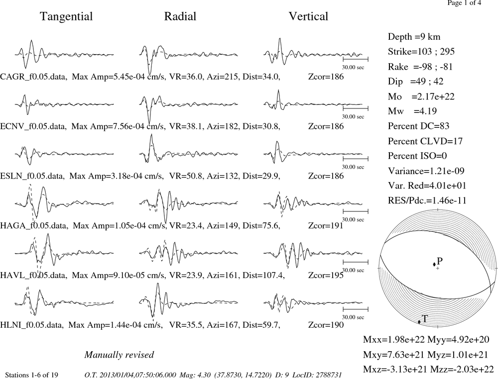
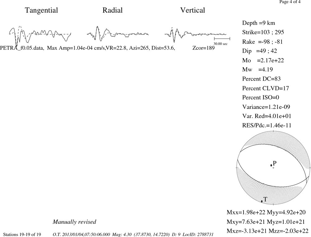
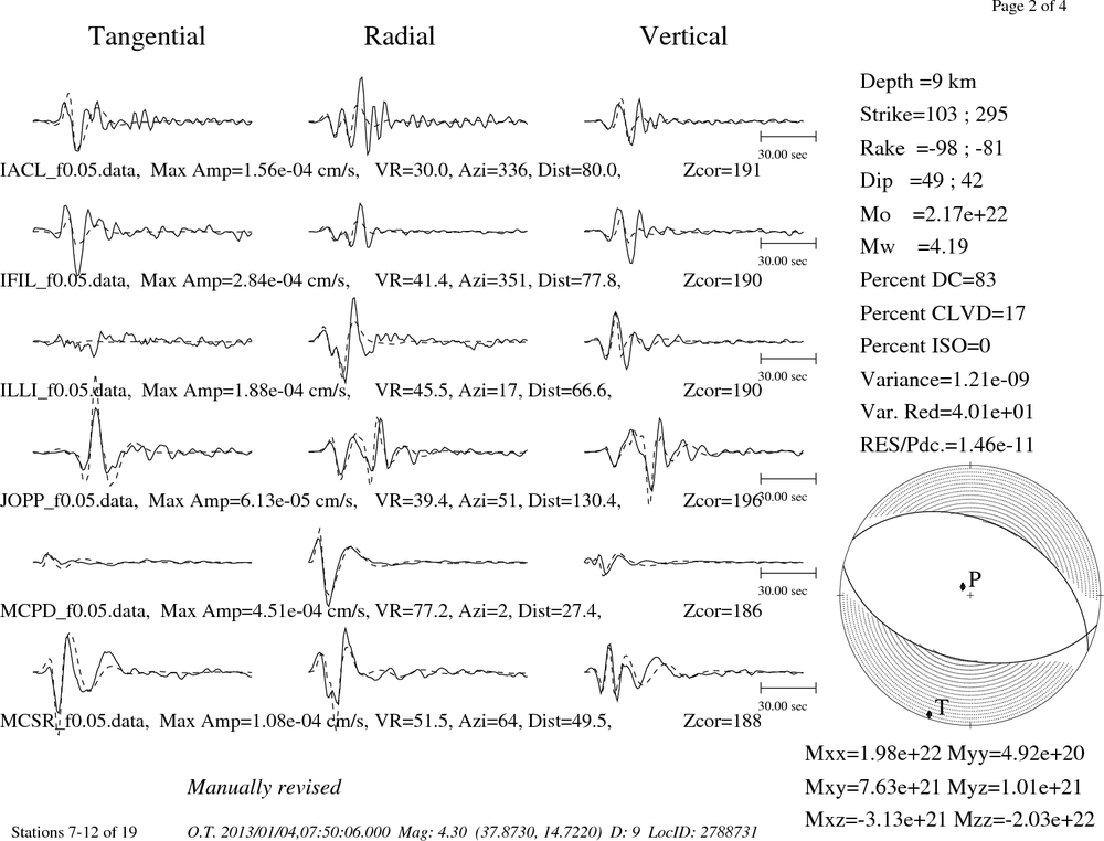
Waveform Inversion

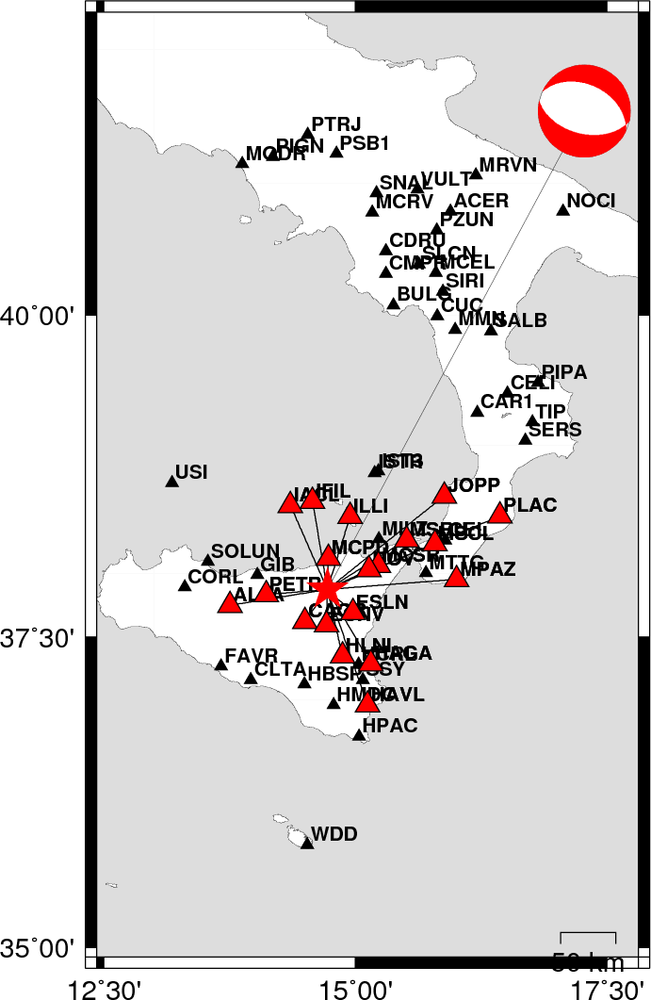
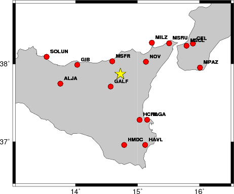
The focal mechanism was determined using broadband seismic waveforms. The location of the event and the and stations used for the waveform inversion are shown in the next figure.

Location of broadband stations used for waveform inversion

The program wvfgrd96 was used with good traces observed at short distance to determine the focal mechanism, depth and seismic moment. This technique requires a high quality signal and well determined velocity model for the Green functions. To the extent that these are the quality data, this type of mechanism should be preferred over the radiation pattern technique which requires the separate step of defining the pressure and tension quadrants and the correct strike.

The observed and predicted traces are filtered using the following gsac commands:

hp c 0.02 n 3
lp c 0.06 n 3

           DEPTH  STK   DIP  RAKE   MW    FIT
WVFGRD96    1.0   290    35   -85   3.88 0.3123
WVFGRD96    2.0   295    30   -75   3.95 0.3151
WVFGRD96    3.0   305    60   -35   3.94 0.3268
WVFGRD96    4.0   310    55   -30   3.96 0.3540
WVFGRD96    5.0   295    20   -75   4.09 0.3838
WVFGRD96    6.0   295    25   -75   4.10 0.4297
WVFGRD96    7.0   295    30   -75   4.10 0.4657
WVFGRD96    8.0   295    35   -75   4.08 0.4868
WVFGRD96    9.0   305    40   -60   4.07 0.4889
WVFGRD96   10.0   305    40   -60   4.07 0.4858
WVFGRD96   11.0   310    40   -55   4.07 0.4772
WVFGRD96   12.0   315    45   -45   4.06 0.4669
WVFGRD96   13.0   315    50   -35   4.06 0.4564
WVFGRD96   14.0   315    55   -30   4.07 0.4476
WVFGRD96   15.0   315    55   -30   4.09 0.4395
WVFGRD96   16.0   315    55   -30   4.10 0.4296
WVFGRD96   17.0   315    55   -30   4.10 0.4186
WVFGRD96   18.0   315    60   -25   4.11 0.4075
WVFGRD96   19.0   315    60   -25   4.11 0.3962
WVFGRD96   20.0   315    60   -25   4.12 0.3843
WVFGRD96   21.0   320    60   -20   4.12 0.3723
WVFGRD96   22.0   320    65   -25   4.12 0.3609
WVFGRD96   23.0   345    55    25   4.10 0.3552
WVFGRD96   24.0   345    55    25   4.11 0.3491
WVFGRD96   25.0   345    55    25   4.11 0.3435
WVFGRD96   26.0   345    55    25   4.12 0.3380
WVFGRD96   27.0   345    55    25   4.13 0.3331
WVFGRD96   28.0   340    60    25   4.14 0.3296
WVFGRD96   29.0   340    60    25   4.15 0.3264

The best solution is

WVFGRD96    9.0   305    40   -60   4.07 0.4889

The mechanism correspond to the best fit is

Figure 1. Waveform inversion focal mechanism

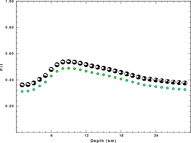
The best fit as a function of depth is given in the following figure:

Figure 2. Depth sensitivity for waveform mechanism

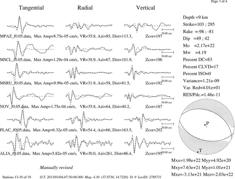
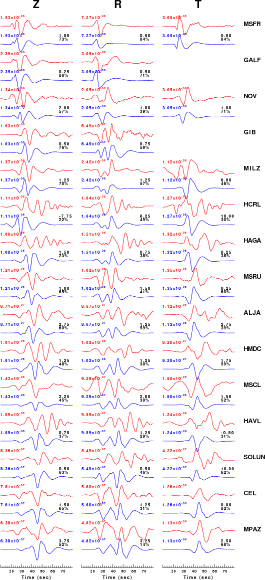
The comparison of the observed and predicted waveforms is given in the next figure. The red traces are the observed and the blue are the predicted. Each observed-predicted component is plotted to the same scale and peak amplitudes are indicated by the numbers to the left of each trace. A pair of numbers is given in black at the right of each predicted traces. The upper number it the time shift required for maximum correlation between the observed and predicted traces. This time shift is required because the synthetics are not computed at exactly the same distance as the observed and because the velocity model used in the predictions may not be perfect. A positive time shift indicates that the prediction is too fast and should be delayed to match the observed trace (shift to the right in this figure). A negative value indicates that the prediction is too slow. The lower number gives the percentage of variance reduction to characterize the individual goodness of fit (100% indicates a perfect fit).

The bandpass filter used in the processing and for the display was

hp c 0.02 n 3
lp c 0.06 n 3

Figure 3. Waveform comparison for selected depth

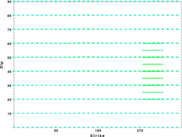
Focal mechanism sensitivity at the preferred depth. The red color indicates a very good fit to thewavefroms. Each solution is plotted as a vector at a given value of strike and dip with the angle of the vector representing the rake angle, measured, with respect to the upward vertical (N) in the figure.

A check on the assumed source location is possible by looking at the time shifts between the observed and predicted traces. The time shifts for waveform matching arise for several reasons:

• The origin time and epicentral distance are incorrect
• The velocity model used for the inversion is incorrect
• The velocity model used to define the P-arrival time is not the same as the velocity model used for the waveform inversion (assuming that the initial trace alignment is based on the P arrival time)

 Time_shift = A + B cos Azimuth + C Sin Azimuth

The time shifts for this inversion lead to the next figure:

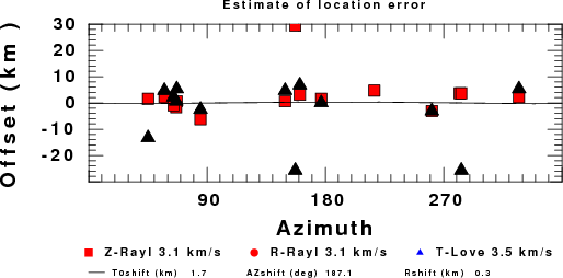
The derived shift in origin time and epicentral coordinates are given at the bottom of the figure.

Discussion

Velocity Model

The nnCIA used for the waveform synthetic seismograms and for the surface wave eigenfunctions and dispersion is as follows:

MODEL.01
C.It. A. Di Luzio et al Earth Plan Lettrs 280 (2009) 1-12 Fig 5. 7-8 MODEL/SURF3
ISOTROPIC
KGS
FLAT EARTH
1-D
CONSTANT VELOCITY
LINE08
LINE09
LINE10
LINE11
      H(KM)   VP(KM/S)   VS(KM/S) RHO(GM/CC)         QP         QS       ETAP       ETAS      FREFP      FREFS
     1.5000     3.7497     2.1436     2.2753  0.500E-02  0.100E-01   0.00       0.00       1.00       1.00    
     3.0000     4.9399     2.8210     2.4858  0.500E-02  0.100E-01   0.00       0.00       1.00       1.00    
     3.0000     6.0129     3.4336     2.7058  0.500E-02  0.100E-01   0.00       0.00       1.00       1.00    
     7.0000     5.5516     3.1475     2.6093  0.167E-02  0.333E-02   0.00       0.00       1.00       1.00    
    15.0000     5.8805     3.3583     2.6770  0.167E-02  0.333E-02   0.00       0.00       1.00       1.00    
     6.0000     7.1059     4.0081     3.0002  0.167E-02  0.333E-02   0.00       0.00       1.00       1.00    
     8.0000     7.1000     3.9864     3.0120  0.167E-02  0.333E-02   0.00       0.00       1.00       1.00    
     0.0000     7.9000     4.4036     3.2760  0.167E-02  0.333E-02   0.00       0.00       1.00       1.00    

Quality Control

Here we tabulate the reasons for not using certain digital data sets

The following stations did not have a valid response files:

DATE=Fri Jan 4 07:20:46 CST 2013