Location

2012/07/09 15:13:43 41.874 12.720 10.0 3.5 Italy

SLU Moment Tensor Solution ENS 2012/07/09 15:13:43:0 41.87 12.72 10.0 3.5 Italy Stations used: IV.ASSB IV.CAMP IV.CERA IV.CERT IV.CESI IV.CESX IV.CING IV.FAGN IV.FDMO IV.FIAM IV.GIUL IV.LAV9 IV.LPEL IV.MA9 IV.MAON IV.MODR IV.MTCE IV.NRCA IV.POFI IV.PTQR IV.SACS IV.SGG IV.T0104 IV.TERO IV.TOLF IV.VVLD Filtering commands used: hp c 0.025 n 3 lp c 0.10 n 3 Best Fitting Double Couple Mo = 2.66e+21 dyne-cm Mw = 3.55 Z = 6 km Plane Strike Dip Rake NP1 341 57 -103 NP2 185 35 -70 Principal Axes: Axis Value Plunge Azimuth T 2.66e+21 11 81 N 0.00e+00 11 348 P -2.66e+21 74 215 Moment Tensor: (dyne-cm) Component Value Mxx -7.28e+19 Mxy 3.10e+20 Mxz 6.68e+20 Myy 2.42e+21 Myz 9.17e+20 Mzz -2.35e+21 #----######### ######--############## #######-------############## ######----------############## #######-------------############## #######---------------############## #######-----------------############## ########------------------############## #######--------------------########## ########---------------------######### T # #######----------------------######### # #######---------- ----------############ #######---------- P ----------############ #######--------- ----------########### #######-----------------------########## #######----------------------######### ######----------------------######## ######--------------------######## #####-------------------###### ######-----------------##### ####---------------### ###----------- Global CMT Convention Moment Tensor: R T P -2.35e+21 6.68e+20 -9.17e+20 6.68e+20 -7.28e+19 -3.10e+20 -9.17e+20 -3.10e+20 2.42e+21 Details of the solution is found at http://www.eas.slu.edu/eqc/eqc_mt/MECH.IT/20120709151343/index.html

Preferred Solution

The preferred solution from an analysis of the surface-wave spectral amplitude radiation pattern, waveform inversion and first motion observations is

      STK = 185
      DIP = 35
     RAKE = -70
       MW = 3.55
       HS = 6.0

The waveform inversion is preferred.

Moment Tensor Comparison

The following compares this source inversion to others

SLU

SLU Moment Tensor Solution ENS 2012/07/09 15:13:43:0 41.87 12.72 10.0 3.5 Italy Stations used: IV.ASSB IV.CAMP IV.CERA IV.CERT IV.CESI IV.CESX IV.CING IV.FAGN IV.FDMO IV.FIAM IV.GIUL IV.LAV9 IV.LPEL IV.MA9 IV.MAON IV.MODR IV.MTCE IV.NRCA IV.POFI IV.PTQR IV.SACS IV.SGG IV.T0104 IV.TERO IV.TOLF IV.VVLD Filtering commands used: hp c 0.025 n 3 lp c 0.10 n 3 Best Fitting Double Couple Mo = 2.66e+21 dyne-cm Mw = 3.55 Z = 6 km Plane Strike Dip Rake NP1 341 57 -103 NP2 185 35 -70 Principal Axes: Axis Value Plunge Azimuth T 2.66e+21 11 81 N 0.00e+00 11 348 P -2.66e+21 74 215 Moment Tensor: (dyne-cm) Component Value Mxx -7.28e+19 Mxy 3.10e+20 Mxz 6.68e+20 Myy 2.42e+21 Myz 9.17e+20 Mzz -2.35e+21 #----######### ######--############## #######-------############## ######----------############## #######-------------############## #######---------------############## #######-----------------############## ########------------------############## #######--------------------########## ########---------------------######### T # #######----------------------######### # #######---------- ----------############ #######---------- P ----------############ #######--------- ----------########### #######-----------------------########## #######----------------------######### ######----------------------######## ######--------------------######## #####-------------------###### ######-----------------##### ####---------------### ###----------- Global CMT Convention Moment Tensor: R T P -2.35e+21 6.68e+20 -9.17e+20 6.68e+20 -7.28e+19 -3.10e+20 -9.17e+20 -3.10e+20 2.42e+21 Details of the solution is found at http://www.eas.slu.edu/eqc/eqc_mt/MECH.IT/20120709151343/index.html

Waveform Inversion

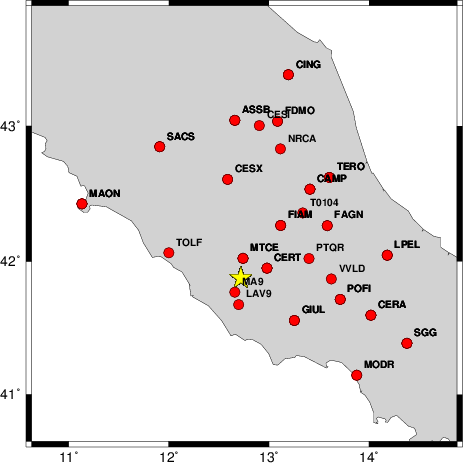
The focal mechanism was determined using broadband seismic waveforms. The location of the event and the and stations used for the waveform inversion are shown in the next figure.

Location of broadband stations used for waveform inversion

The program wvfgrd96 was used with good traces observed at short distance to determine the focal mechanism, depth and seismic moment. This technique requires a high quality signal and well determined velocity model for the Green functions. To the extent that these are the quality data, this type of mechanism should be preferred over the radiation pattern technique which requires the separate step of defining the pressure and tension quadrants and the correct strike.

The observed and predicted traces are filtered using the following gsac commands:

hp c 0.025 n 3
lp c 0.10 n 3

The results of this grid search from 0.5 to 19 km depth are as follow:

           DEPTH  STK   DIP  RAKE   MW    FIT
WVFGRD96    1.0   210    40   -30   3.32 0.4210
WVFGRD96    2.0   205    35   -30   3.39 0.4626
WVFGRD96    3.0   200    30   -45   3.43 0.5139
WVFGRD96    4.0   185    30   -70   3.46 0.5670
WVFGRD96    5.0   185    30   -70   3.55 0.6090
WVFGRD96    6.0   185    35   -70   3.55 0.6196
WVFGRD96    7.0   185    35   -65   3.53 0.6009
WVFGRD96    8.0   195    40   -55   3.48 0.5576
WVFGRD96    9.0   220    65    25   3.49 0.5352
WVFGRD96   10.0   215    70    25   3.51 0.5216
WVFGRD96   11.0   215    70    20   3.51 0.5060
WVFGRD96   12.0   215    70    20   3.53 0.4876
WVFGRD96   13.0   215    70    20   3.54 0.4677
WVFGRD96   14.0   220    65    20   3.54 0.4511
WVFGRD96   15.0   220    60    25   3.56 0.4267
WVFGRD96   16.0   220    60    20   3.56 0.4089
WVFGRD96   17.0   220    60    20   3.57 0.3918
WVFGRD96   18.0   220    60    20   3.58 0.3753
WVFGRD96   19.0   220    60    20   3.59 0.3601
WVFGRD96   20.0   220    60    20   3.59 0.3455
WVFGRD96   21.0   220    60    20   3.60 0.3316
WVFGRD96   22.0   220    60    20   3.61 0.3178
WVFGRD96   23.0   215    65    15   3.62 0.3066
WVFGRD96   24.0   215    65    15   3.62 0.2973
WVFGRD96   25.0   205    65   -25   3.61 0.2896
WVFGRD96   26.0   305    75   -30   3.62 0.2908
WVFGRD96   27.0   305    75   -25   3.63 0.2935
WVFGRD96   28.0   125    65   -20   3.68 0.2972
WVFGRD96   29.0   125    70   -20   3.70 0.3059

The best solution is

WVFGRD96    6.0   185    35   -70   3.55 0.6196

The mechanism correspond to the best fit is

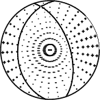
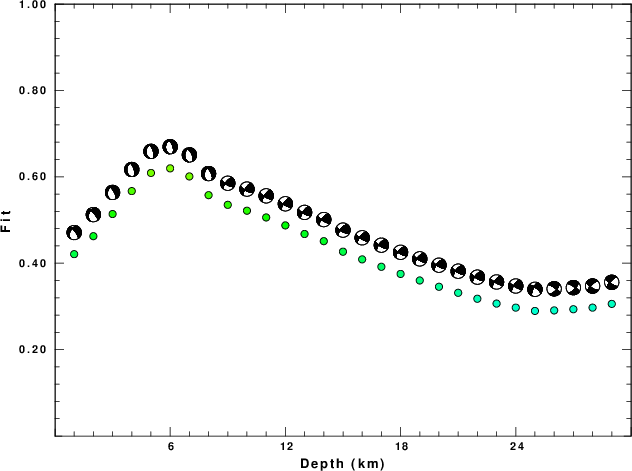
Figure 1. Waveform inversion focal mechanism

The best fit as a function of depth is given in the following figure:

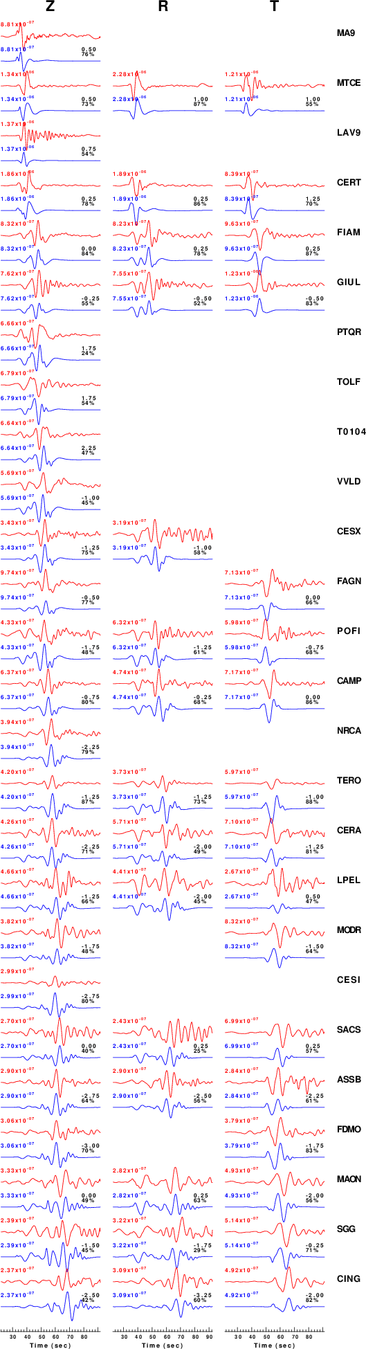
Figure 2. Depth sensitivity for waveform mechanism

The comparison of the observed and predicted waveforms is given in the next figure. The red traces are the observed and the blue are the predicted. Each observed-predicted component is plotted to the same scale and peak amplitudes are indicated by the numbers to the left of each trace. A pair of numbers is given in black at the right of each predicted traces. The upper number it the time shift required for maximum correlation between the observed and predicted traces. This time shift is required because the synthetics are not computed at exactly the same distance as the observed and because the velocity model used in the predictions may not be perfect. A positive time shift indicates that the prediction is too fast and should be delayed to match the observed trace (shift to the right in this figure). A negative value indicates that the prediction is too slow. The lower number gives the percentage of variance reduction to characterize the individual goodness of fit (100% indicates a perfect fit).

The bandpass filter used in the processing and for the display was

hp c 0.025 n 3
lp c 0.10 n 3

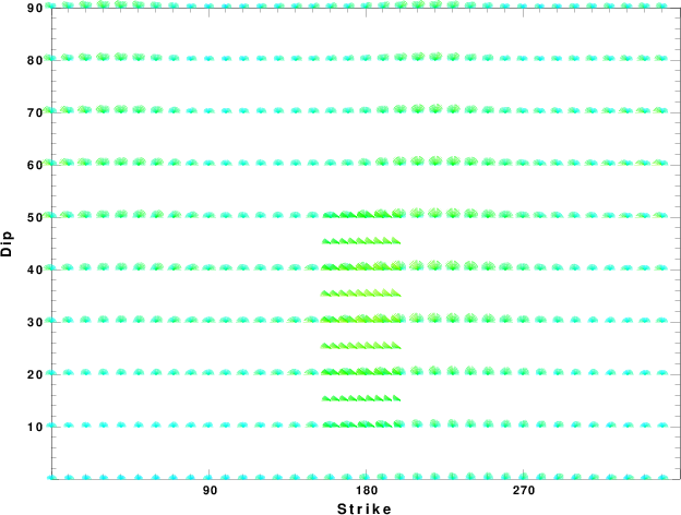
Figure 3. Waveform comparison for selected depth

Focal mechanism sensitivity at the preferred depth. The red color indicates a very good fit to thewavefroms. Each solution is plotted as a vector at a given value of strike and dip with the angle of the vector representing the rake angle, measured, with respect to the upward vertical (N) in the figure.

A check on the assumed source location is possible by looking at the time shifts between the observed and predicted traces. The time shifts for waveform matching arise for several reasons:

The origin time and epicentral distance are incorrect
The velocity model used for the inversion is incorrect
The velocity model used to define the P-arrival time is not the same as the velocity model used for the waveform inversion (assuming that the initial trace alignment is based on the P arrival time)

Assuming only a mislocation, the time shifts are fit to a functional form:

 Time_shift = A + B cos Azimuth + C Sin Azimuth

The time shifts for this inversion lead to the next figure:

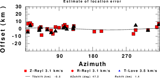
The derived shift in origin time and epicentral coordinates are given at the bottom of the figure.

Discussion

Velocity Model

The nnCIA used for the waveform synthetic seismograms and for the surface wave eigenfunctions and dispersion is as follows:

MODEL.01
C.It. A. Di Luzio et al Earth Plan Lettrs 280 (2009) 1-12 Fig 5. 7-8 MODEL/SURF3
ISOTROPIC
KGS
FLAT EARTH
1-D
CONSTANT VELOCITY
LINE08
LINE09
LINE10
LINE11
      H(KM)   VP(KM/S)   VS(KM/S) RHO(GM/CC)         QP         QS       ETAP       ETAS      FREFP      FREFS
     1.5000     3.7497     2.1436     2.2753  0.500E-02  0.100E-01   0.00       0.00       1.00       1.00    
     3.0000     4.9399     2.8210     2.4858  0.500E-02  0.100E-01   0.00       0.00       1.00       1.00    
     3.0000     6.0129     3.4336     2.7058  0.500E-02  0.100E-01   0.00       0.00       1.00       1.00    
     7.0000     5.5516     3.1475     2.6093  0.167E-02  0.333E-02   0.00       0.00       1.00       1.00    
    15.0000     5.8805     3.3583     2.6770  0.167E-02  0.333E-02   0.00       0.00       1.00       1.00    
     6.0000     7.1059     4.0081     3.0002  0.167E-02  0.333E-02   0.00       0.00       1.00       1.00    
     8.0000     7.1000     3.9864     3.0120  0.167E-02  0.333E-02   0.00       0.00       1.00       1.00    
     0.0000     7.9000     4.4036     3.2760  0.167E-02  0.333E-02   0.00       0.00       1.00       1.00

Quality Control

Here we tabulate the reasons for not using certain digital data sets

The following stations did not have a valid response files:

DATE=Mon Jul 9 21:42:20 CDT 2012

Last Changed 2012/07/09