2012/06/25 01:39:16 41.935 15.501 4.8 3.4 Italy
 SLU Moment Tensor Solution
 ENS  2012/06/25 01:39:16:0  41.94   15.50   4.8 3.4 Italy

 Stations used:
   IV.ACER IV.AMUR IV.BSSO IV.CDRU IV.CMPR IV.FRES IV.GATE
   IV.MCRV IV.MELA IV.MGR IV.MIDA IV.MMN IV.MODR IV.MRB1
   IV.MRLC IV.MRVN IV.MSAG IV.NOCI IV.PAOL IV.PTRJ IV.SACR
   IV.SALB IV.SGG IV.SGRT IV.SGTA IV.SLCN IV.TRIV IV.VULT
   MN.AQU MN.CUC

 Filtering commands used:
   hp c 0.025 n 3
   lp c 0.08 n 3

 Best Fitting Double Couple
  Mo = 7.94e+20 dyne-cm
  Mw = 3.20
  Z  = 16 km
  Plane   Strike  Dip  Rake
   NP1      287    76   104
   NP2       60    20    45
  Principal Axes:
   Axis    Value   Plunge  Azimuth
    T   7.94e+20     57     215
    N   0.00e+00     14     103
    P  -7.94e+20     30       5

 Moment Tensor: (dyne-cm)
    Component   Value
       Mxx    -4.37e+20
       Mxy     6.03e+19
       Mxz    -6.37e+20
       Myy     7.61e+19
       Myz    -2.42e+20
       Mzz     3.61e+20


                     --------------
                 ----------------------
              --------------   -----------
             --------------- P ------------
           -----------------   --------------
          ------------------------------------
         --------------------------------------
        ---------------------------------------#
        #################----------------------#
       ########################----------------##
       #############################-----------##
       #################################-------##
       #####################################--###
        ##############   ####################-##
        ############## T ###################----
         #############   ##################----
          ################################----
           -############################-----
             -########################-----
              ---#################--------
                 ----------------------
                     --------------


 Global CMT Convention Moment Tensor:
      R          T          P
  3.61e+20  -6.37e+20   2.42e+20
 -6.37e+20  -4.37e+20  -6.03e+19
  2.42e+20  -6.03e+19   7.61e+19


Details of the solution is found at

http://www.eas.slu.edu/eqc/eqc_mt/MECH.IT/20120625013916/index.html
|
      STK = 60
      DIP = 20
     RAKE = 45
       MW = 3.20
       HS = 16.0
The waveform inversion is preferred.
The following compares this source inversion to others
 SLU Moment Tensor Solution
 ENS  2012/06/25 01:39:16:0  41.94   15.50   4.8 3.4 Italy

 Stations used:
   IV.ACER IV.AMUR IV.BSSO IV.CDRU IV.CMPR IV.FRES IV.GATE
   IV.MCRV IV.MELA IV.MGR IV.MIDA IV.MMN IV.MODR IV.MRB1
   IV.MRLC IV.MRVN IV.MSAG IV.NOCI IV.PAOL IV.PTRJ IV.SACR
   IV.SALB IV.SGG IV.SGRT IV.SGTA IV.SLCN IV.TRIV IV.VULT
   MN.AQU MN.CUC

 Filtering commands used:
   hp c 0.025 n 3
   lp c 0.08 n 3

 Best Fitting Double Couple
  Mo = 7.94e+20 dyne-cm
  Mw = 3.20
  Z  = 16 km
  Plane   Strike  Dip  Rake
   NP1      287    76   104
   NP2       60    20    45
  Principal Axes:
   Axis    Value   Plunge  Azimuth
    T   7.94e+20     57     215
    N   0.00e+00     14     103
    P  -7.94e+20     30       5

 Moment Tensor: (dyne-cm)
    Component   Value
       Mxx    -4.37e+20
       Mxy     6.03e+19
       Mxz    -6.37e+20
       Myy     7.61e+19
       Myz    -2.42e+20
       Mzz     3.61e+20


                     --------------
                 ----------------------
              --------------   -----------
             --------------- P ------------
           -----------------   --------------
          ------------------------------------
         --------------------------------------
        ---------------------------------------#
        #################----------------------#
       ########################----------------##
       #############################-----------##
       #################################-------##
       #####################################--###
        ##############   ####################-##
        ############## T ###################----
         #############   ##################----
          ################################----
           -############################-----
             -########################-----
              ---#################--------
                 ----------------------
                     --------------


 Global CMT Convention Moment Tensor:
      R          T          P
  3.61e+20  -6.37e+20   2.42e+20
 -6.37e+20  -4.37e+20  -6.03e+19
  2.42e+20  -6.03e+19   7.61e+19


Details of the solution is found at

http://www.eas.slu.edu/eqc/eqc_mt/MECH.IT/20120625013916/index.html
|
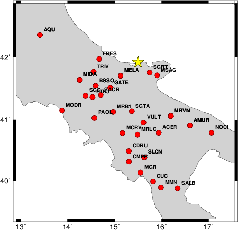
The focal mechanism was determined using broadband seismic waveforms. The location of the event and the and stations used for the waveform inversion are shown in the next figure.
|
|
|
|
The program wvfgrd96 was used with good traces observed at short distance to determine the focal mechanism, depth and seismic moment. This technique requires a high quality signal and well determined velocity model for the Green functions. To the extent that these are the quality data, this type of mechanism should be preferred over the radiation pattern technique which requires the separate step of defining the pressure and tension quadrants and the correct strike.
The observed and predicted traces are filtered using the following gsac commands:
hp c 0.025 n 3
lp c 0.08 n 3
The results of this grid search from 0.5 to 19 km depth are as follow:
           DEPTH  STK   DIP  RAKE   MW    FIT
WVFGRD96    1.0   120    45   -90   2.98 0.3635
WVFGRD96    2.0   305    45   -90   3.04 0.3376
WVFGRD96    3.0    20    80    10   3.08 0.2586
WVFGRD96    4.0   200    55     5   3.08 0.2675
WVFGRD96    5.0   180    25   -30   3.12 0.3000
WVFGRD96    6.0   185    25   -20   3.11 0.3267
WVFGRD96    7.0    20    10    -5   3.10 0.3558
WVFGRD96    8.0    45    15    25   3.06 0.3883
WVFGRD96    9.0    50    15    30   3.08 0.4133
WVFGRD96   10.0    60    15    40   3.09 0.4338
WVFGRD96   11.0    60    15    40   3.10 0.4518
WVFGRD96   12.0    55    20    35   3.12 0.4653
WVFGRD96   13.0    50    25    35   3.14 0.4767
WVFGRD96   14.0    50    25    35   3.15 0.4843
WVFGRD96   15.0    60    20    45   3.19 0.4877
WVFGRD96   16.0    60    20    45   3.20 0.4900
WVFGRD96   17.0    55    20    35   3.20 0.4897
WVFGRD96   18.0    55    20    40   3.22 0.4876
WVFGRD96   19.0    50    25    35   3.24 0.4828
WVFGRD96   20.0    45    25    30   3.25 0.4758
WVFGRD96   21.0    45    25    30   3.26 0.4669
WVFGRD96   22.0    45    25    30   3.26 0.4568
WVFGRD96   23.0    45    25    30   3.27 0.4447
WVFGRD96   24.0    50    25    30   3.27 0.4320
WVFGRD96   25.0    50    25    30   3.28 0.4182
WVFGRD96   26.0    45    30    30   3.29 0.4014
WVFGRD96   27.0    45    30    30   3.30 0.3880
WVFGRD96   28.0    45    30    30   3.30 0.3753
WVFGRD96   29.0    50    30    35   3.30 0.3674
The best solution is
WVFGRD96 16.0 60 20 45 3.20 0.4900
The mechanism correspond to the best fit is
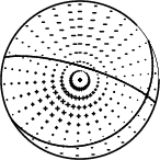
|
|
|
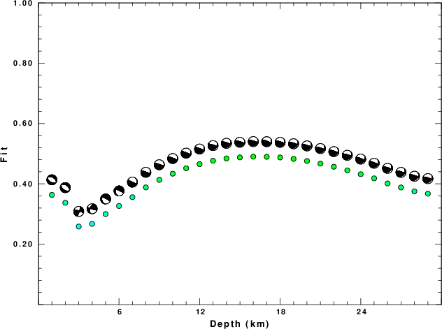
The best fit as a function of depth is given in the following figure:
|
|
|
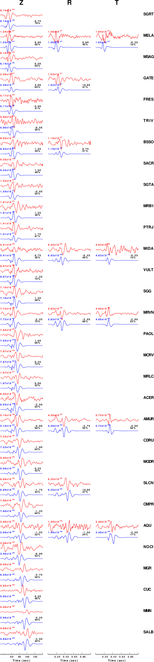
The comparison of the observed and predicted waveforms is given in the next figure. The red traces are the observed and the blue are the predicted. Each observed-predicted component is plotted to the same scale and peak amplitudes are indicated by the numbers to the left of each trace. A pair of numbers is given in black at the right of each predicted traces. The upper number it the time shift required for maximum correlation between the observed and predicted traces. This time shift is required because the synthetics are not computed at exactly the same distance as the observed and because the velocity model used in the predictions may not be perfect. A positive time shift indicates that the prediction is too fast and should be delayed to match the observed trace (shift to the right in this figure). A negative value indicates that the prediction is too slow. The lower number gives the percentage of variance reduction to characterize the individual goodness of fit (100% indicates a perfect fit).
The bandpass filter used in the processing and for the display was
hp c 0.025 n 3
lp c 0.08 n 3
|
|
|
|
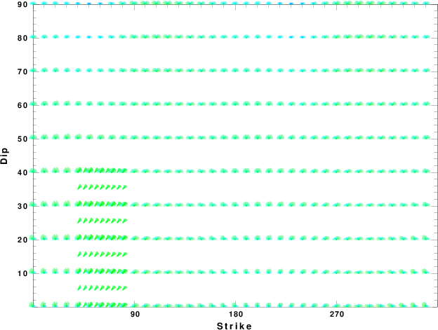
| Focal mechanism sensitivity at the preferred depth. The red color indicates a very good fit to thewavefroms. Each solution is plotted as a vector at a given value of strike and dip with the angle of the vector representing the rake angle, measured, with respect to the upward vertical (N) in the figure. |
A check on the assumed source location is possible by looking at the time shifts between the observed and predicted traces. The time shifts for waveform matching arise for several reasons:
Time_shift = A + B cos Azimuth + C Sin Azimuth
The time shifts for this inversion lead to the next figure:
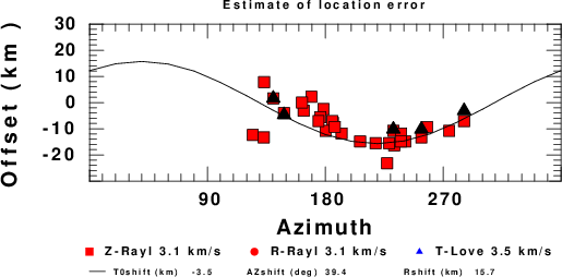
The derived shift in origin time and epicentral coordinates are given at the bottom of the figure.
The nnCIA used for the waveform synthetic seismograms and for the surface wave eigenfunctions and dispersion is as follows:
MODEL.01
C.It. A. Di Luzio et al Earth Plan Lettrs 280 (2009) 1-12 Fig 5. 7-8 MODEL/SURF3
ISOTROPIC
KGS
FLAT EARTH
1-D
CONSTANT VELOCITY
LINE08
LINE09
LINE10
LINE11
      H(KM)   VP(KM/S)   VS(KM/S) RHO(GM/CC)         QP         QS       ETAP       ETAS      FREFP      FREFS
     1.5000     3.7497     2.1436     2.2753  0.500E-02  0.100E-01   0.00       0.00       1.00       1.00
     3.0000     4.9399     2.8210     2.4858  0.500E-02  0.100E-01   0.00       0.00       1.00       1.00
     3.0000     6.0129     3.4336     2.7058  0.500E-02  0.100E-01   0.00       0.00       1.00       1.00
     7.0000     5.5516     3.1475     2.6093  0.167E-02  0.333E-02   0.00       0.00       1.00       1.00
    15.0000     5.8805     3.3583     2.6770  0.167E-02  0.333E-02   0.00       0.00       1.00       1.00
     6.0000     7.1059     4.0081     3.0002  0.167E-02  0.333E-02   0.00       0.00       1.00       1.00
     8.0000     7.1000     3.9864     3.0120  0.167E-02  0.333E-02   0.00       0.00       1.00       1.00
     0.0000     7.9000     4.4036     3.2760  0.167E-02  0.333E-02   0.00       0.00       1.00       1.00
Here we tabulate the reasons for not using certain digital data sets
The following stations did not have a valid response files:
DATE=Tue Jun 26 02:39:38 CDT 2012