Location
2012/05/28 01:06:27 39.859 16.118 3.0 4.3 Italy
Arrival Times (from USGS)
Arrival time list
Felt Map
USGS Felt map for this earthquake
USGS Felt reports page for
Focal Mechanism
 SLU Moment Tensor Solution
 ENS  2012/05/28 01:06:27:0  39.86   16.12   3.0 4.3 Italy

 Stations used:
   BA.PZUN GE.MATE IV.BULG IV.CAR1 IV.CDRU IV.CERA IV.CMPR
   IV.MCEL IV.MCRV IV.MELA IV.MGR IV.MIDA IV.MRB1 IV.MRVN
   IV.MSCL IV.MTSN IV.NOCI IV.ORI IV.PIPA IV.PLAC IV.RNI2
   IV.SALB IV.SGG IV.SGRT

 Filtering commands used:
   hp c 0.02 n 3
   lp c 0.05 n 3

 Best Fitting Double Couple
  Mo = 3.20e+22 dyne-cm
  Mw = 4.27
  Z  = 5 km
  Plane   Strike  Dip  Rake
   NP1      150    45   -90
   NP2      330    45   -90
  Principal Axes:
   Axis    Value   Plunge  Azimuth
    T   3.20e+22     -0     240
    N   0.00e+00     -0     150
    P  -3.20e+22     90       5

 Moment Tensor: (dyne-cm)
    Component   Value
       Mxx     8.00e+21
       Mxy     1.39e+22
       Mxz     1.56e+15
       Myy     2.40e+22
       Myz     7.17e+14
       Mzz    -3.20e+22


                     ##############
                 ------################
              ##-----------###############
             ###--------------#############
           ####------------------############
          #####-------------------############
         ######---------------------###########
        #######----------------------###########
        #######------------   --------##########
       ########------------ P ---------##########
       #########-----------   ----------#########
       #########------------------------#########
       ##########------------------------########
        ##########-----------------------#######
        ###########----------------------#######
            ########---------------------######
          T ##########-------------------#####
            ###########------------------####
             #############--------------###
              ###############-----------##
                 ################------
                     ##############


 Global CMT Convention Moment Tensor:
      R          T          P
 -3.20e+22   1.56e+15  -7.17e+14
  1.56e+15   8.00e+21  -1.39e+22
 -7.17e+14  -1.39e+22   2.40e+22


Details of the solution is found at

http://www.eas.slu.edu/eqc/eqc_mt/MECH.IT/20120528010627/index.html
|
Preferred Solution
The preferred solution from an analysis of the surface-wave spectral amplitude radiation pattern, waveform inversion and first motion observations is
      STK = 330
      DIP = 45
     RAKE = -90
       MW = 4.27
       HS = 5.0
The waveform inversion is preferred.
Moment Tensor Comparison
The following compares this source inversion to others
| SLU |
INGVTDMT |
 SLU Moment Tensor Solution
 ENS  2012/05/28 01:06:27:0  39.86   16.12   3.0 4.3 Italy

 Stations used:
   BA.PZUN GE.MATE IV.BULG IV.CAR1 IV.CDRU IV.CERA IV.CMPR
   IV.MCEL IV.MCRV IV.MELA IV.MGR IV.MIDA IV.MRB1 IV.MRVN
   IV.MSCL IV.MTSN IV.NOCI IV.ORI IV.PIPA IV.PLAC IV.RNI2
   IV.SALB IV.SGG IV.SGRT

 Filtering commands used:
   hp c 0.02 n 3
   lp c 0.05 n 3

 Best Fitting Double Couple
  Mo = 3.20e+22 dyne-cm
  Mw = 4.27
  Z  = 5 km
  Plane   Strike  Dip  Rake
   NP1      150    45   -90
   NP2      330    45   -90
  Principal Axes:
   Axis    Value   Plunge  Azimuth
    T   3.20e+22     -0     240
    N   0.00e+00     -0     150
    P  -3.20e+22     90       5

 Moment Tensor: (dyne-cm)
    Component   Value
       Mxx     8.00e+21
       Mxy     1.39e+22
       Mxz     1.56e+15
       Myy     2.40e+22
       Myz     7.17e+14
       Mzz    -3.20e+22


                     ##############
                 ------################
              ##-----------###############
             ###--------------#############
           ####------------------############
          #####-------------------############
         ######---------------------###########
        #######----------------------###########
        #######------------   --------##########
       ########------------ P ---------##########
       #########-----------   ----------#########
       #########------------------------#########
       ##########------------------------########
        ##########-----------------------#######
        ###########----------------------#######
            ########---------------------######
          T ##########-------------------#####
            ###########------------------####
             #############--------------###
              ###############-----------##
                 ################------
                     ##############


 Global CMT Convention Moment Tensor:
      R          T          P
 -3.20e+22   1.56e+15  -7.17e+14
  1.56e+15   8.00e+21  -1.39e+22
 -7.17e+14  -1.39e+22   2.40e+22


Details of the solution is found at

http://www.eas.slu.edu/eqc/eqc_mt/MECH.IT/20120528010627/index.html
|
|
Waveform Inversion
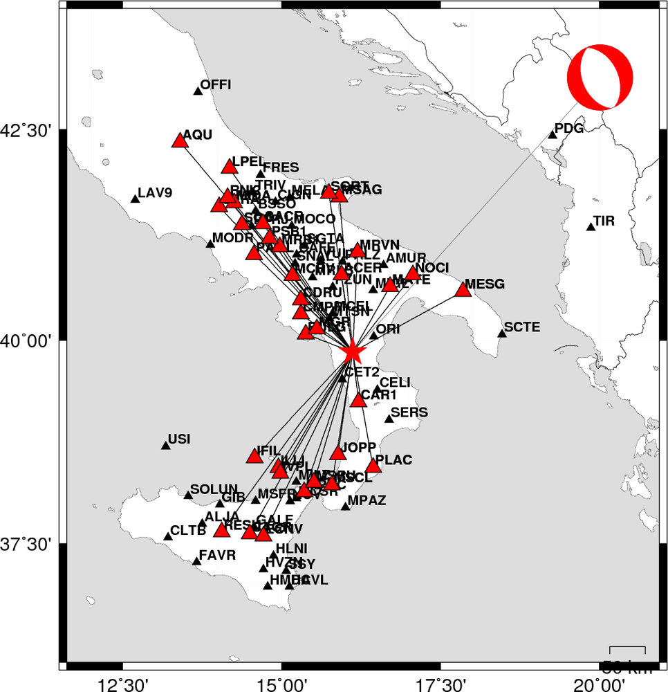
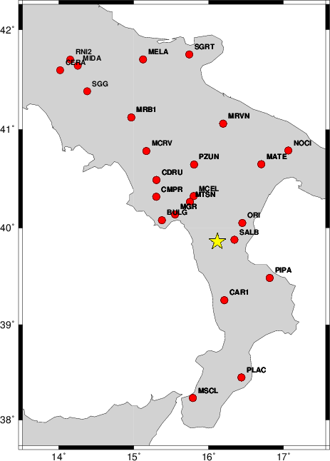
The focal mechanism was determined using broadband seismic waveforms. The location of the event and the
and stations used for the waveform inversion are shown in the next figure.
|
|
Location of broadband stations used for waveform inversion
|
The program wvfgrd96 was used with good traces observed at short distance to determine the focal mechanism, depth and seismic moment. This technique requires a high quality signal and well determined velocity model for the Green functions. To the extent that these are the quality data, this type of mechanism should be preferred over the radiation pattern technique which requires the separate step of defining the pressure and tension quadrants and the correct strike.
The observed and predicted traces are filtered using the following gsac commands:
hp c 0.02 n 3
lp c 0.05 n 3
The results of this grid search from 0.5 to 19 km depth are as follow:
           DEPTH  STK   DIP  RAKE   MW    FIT
WVFGRD96    1.0   335    45   -85   4.13 0.4917
WVFGRD96    2.0   330    45   -90   4.20 0.5431
WVFGRD96    3.0   150    45   -90   4.24 0.5405
WVFGRD96    4.0   150    45   -90   4.26 0.4905
WVFGRD96    5.0   145    45   -95   4.30 0.5149
WVFGRD96    6.0   330    50   -90   4.28 0.4278
WVFGRD96    7.0   180    55   -50   4.20 0.3888
WVFGRD96    8.0   185    45   -35   4.17 0.3897
WVFGRD96    9.0   185    45   -35   4.17 0.3959
WVFGRD96   10.0   185    45   -35   4.17 0.4021
WVFGRD96   11.0   185    45   -35   4.17 0.4071
WVFGRD96   12.0   335    25   -85   4.23 0.4147
WVFGRD96   13.0   340    25   -80   4.23 0.4246
WVFGRD96   14.0   340    25   -80   4.24 0.4335
WVFGRD96   15.0   340    25   -80   4.27 0.4451
WVFGRD96   16.0   345    25   -75   4.27 0.4520
WVFGRD96   17.0   345    25   -75   4.27 0.4568
WVFGRD96   18.0   350    25   -70   4.28 0.4604
WVFGRD96   19.0   350    25   -70   4.28 0.4636
WVFGRD96   20.0   350    25   -70   4.29 0.4655
WVFGRD96   21.0   355    25   -65   4.29 0.4671
WVFGRD96   22.0   355    25   -65   4.30 0.4680
WVFGRD96   23.0   355    25   -65   4.30 0.4685
WVFGRD96   24.0   355    25   -65   4.31 0.4672
WVFGRD96   25.0   355    25   -65   4.31 0.4658
WVFGRD96   26.0    15    55    25   4.27 0.4644
WVFGRD96   27.0    15    55    25   4.28 0.4657
WVFGRD96   28.0    15    55    25   4.30 0.4666
WVFGRD96   29.0    15    55    25   4.31 0.4667
The best solution is
WVFGRD96 2.0 330 45 -90 4.20 0.5431
The mechanism correspond to the best fit is
|
|
Figure 1. Waveform inversion focal mechanism
|
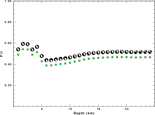
The best fit as a function of depth is given in the following figure:
|
|
Figure 2. Depth sensitivity for waveform mechanism
|
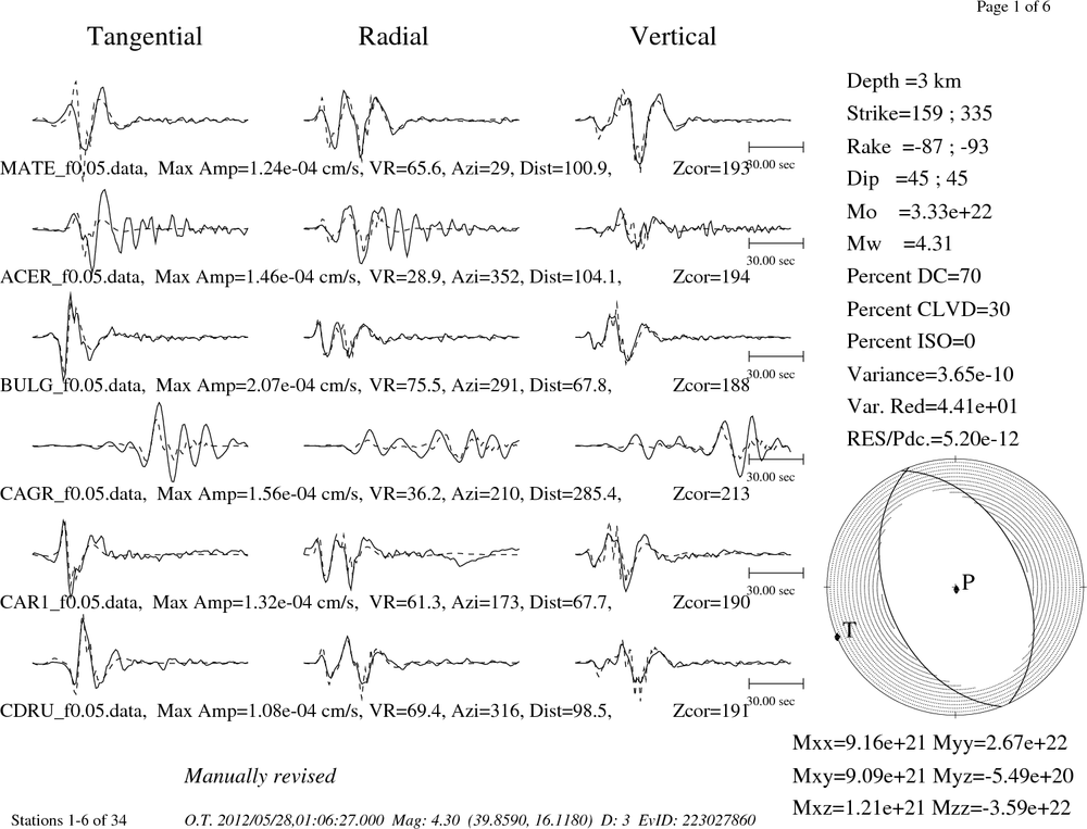
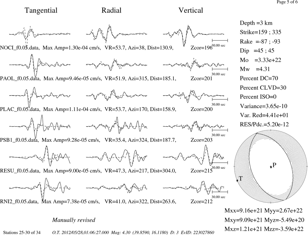
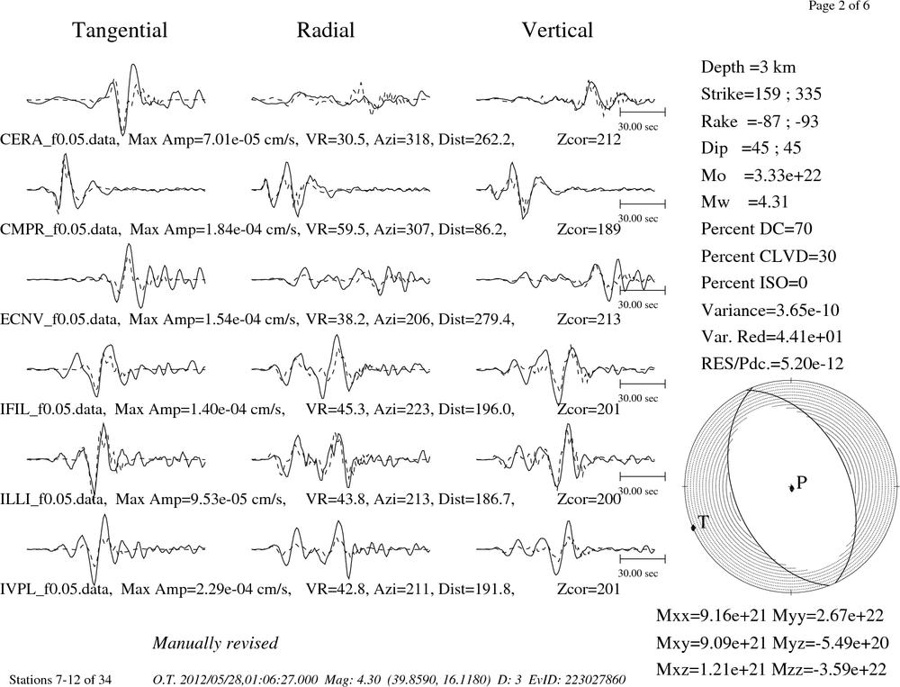
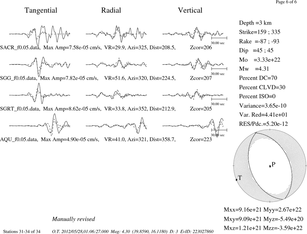
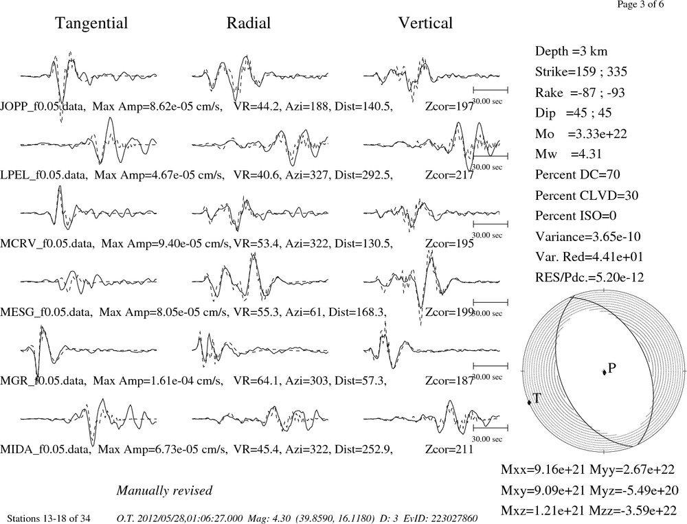
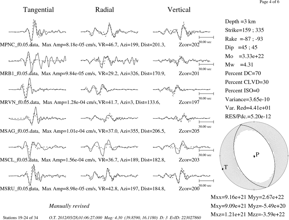
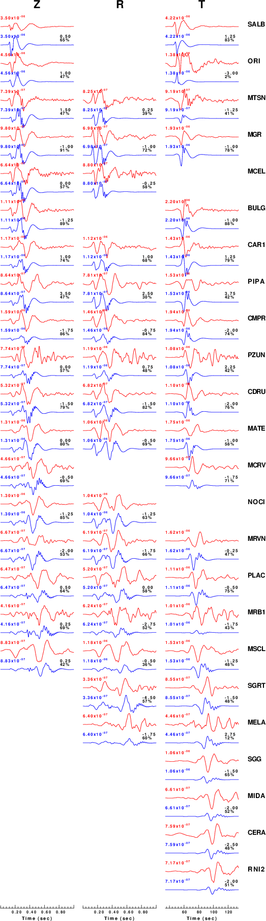
The comparison of the observed and predicted waveforms is given in the next figure. The red traces are the observed and the blue are the predicted.
Each observed-predicted component is plotted to the same scale and peak amplitudes are indicated by the numbers to the left of each trace. A pair of numbers is given in black at the right of each predicted traces. The upper number it the time shift required for maximum correlation between the observed and predicted traces. This time shift is required because the synthetics are not computed at exactly the same distance as the observed and because the velocity model used in the predictions may not be perfect.
A positive time shift indicates that the prediction is too fast and should be delayed to match the observed trace (shift to the right in this figure). A negative value indicates that the prediction is too slow. The lower number gives the percentage of variance reduction to characterize the individual goodness of fit (100% indicates a perfect fit).
The bandpass filter used in the processing and for the display was
hp c 0.02 n 3
lp c 0.05 n 3
|
|
Figure 3. Waveform comparison for selected depth
|
|
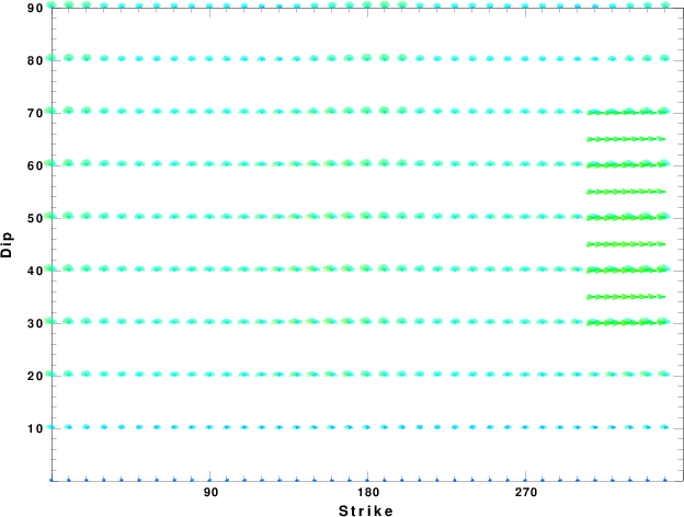
|
Focal mechanism sensitivity at the preferred depth. The red color indicates a very good fit to thewavefroms.
Each solution is plotted as a vector at a given value of strike and dip with the angle of the vector representing the rake angle, measured, with respect to the upward vertical (N) in the figure.
|
A check on the assumed source location is possible by looking at the time shifts between the observed and predicted traces. The time shifts for waveform matching arise for several reasons:
- The origin time and epicentral distance are incorrect
- The velocity model used for the inversion is incorrect
- The velocity model used to define the P-arrival time is not the
same as the velocity model used for the waveform inversion
(assuming that the initial trace alignment is based on the
P arrival time)
Assuming only a mislocation, the time shifts are fit to a functional form:
Time_shift = A + B cos Azimuth + C Sin Azimuth
The time shifts for this inversion lead to the next figure:
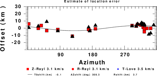
The derived shift in origin time and epicentral coordinates are given at the bottom of the figure.
Discussion
Velocity Model
The nnCIA used for the waveform synthetic seismograms and for the surface wave eigenfunctions and dispersion is as follows:
MODEL.01
C.It. A. Di Luzio et al Earth Plan Lettrs 280 (2009) 1-12 Fig 5. 7-8 MODEL/SURF3
ISOTROPIC
KGS
FLAT EARTH
1-D
CONSTANT VELOCITY
LINE08
LINE09
LINE10
LINE11
      H(KM)   VP(KM/S)   VS(KM/S) RHO(GM/CC)         QP         QS       ETAP       ETAS      FREFP      FREFS
     1.5000     3.7497     2.1436     2.2753  0.500E-02  0.100E-01   0.00       0.00       1.00       1.00
     3.0000     4.9399     2.8210     2.4858  0.500E-02  0.100E-01   0.00       0.00       1.00       1.00
     3.0000     6.0129     3.4336     2.7058  0.500E-02  0.100E-01   0.00       0.00       1.00       1.00
     7.0000     5.5516     3.1475     2.6093  0.167E-02  0.333E-02   0.00       0.00       1.00       1.00
    15.0000     5.8805     3.3583     2.6770  0.167E-02  0.333E-02   0.00       0.00       1.00       1.00
     6.0000     7.1059     4.0081     3.0002  0.167E-02  0.333E-02   0.00       0.00       1.00       1.00
     8.0000     7.1000     3.9864     3.0120  0.167E-02  0.333E-02   0.00       0.00       1.00       1.00
     0.0000     7.9000     4.4036     3.2760  0.167E-02  0.333E-02   0.00       0.00       1.00       1.00
Quality Control
Here we tabulate the reasons for not using certain digital data sets
The following stations did not have a valid response files:
DATE=Mon May 28 11:55:56 CDT 2012
Last Changed 2012/05/28