Location
2012/05/20 02:03:52 44.890 11.230 6.3 5.9 Italy
Arrival Times (from USGS)
Arrival time list
Felt Map
USGS Felt map for this earthquake
USGS Felt reports page for
Focal Mechanism
 SLU Moment Tensor Solution
 ENS  2012/05/20 02:03:52:0  44.89   11.23   6.3 5.9 Italy

 Stations used:
   GU.PCP GU.POPM IV.AOI IV.ARVD IV.ATVO IV.BDI IV.CESI
   IV.CING IV.CRMI IV.FDMO IV.FIR IV.FNVD IV.FROS IV.FSSB
   IV.FVI IV.GUMA IV.LATE IV.MCIV IV.MONC IV.MSSA IV.MURB
   IV.PLMA IV.PRMA IV.QLNO IV.ROVR IV.SACS IV.SALO IV.SNTG
   IV.SSFR IV.STAL IV.TEOL IV.TRIF IV.VARE MN.TUE NI.CGRP
   NI.SABO NI.VINO

 Filtering commands used:
   hp c 0.01 n 3
   lp c 0.04 n 3

 Best Fitting Double Couple
  Mo = 1.02e+25 dyne-cm
  Mw = 5.94
  Z  = 5 km
  Plane   Strike  Dip  Rake
   NP1      278    45    85
   NP2      105    45    95
  Principal Axes:
   Axis    Value   Plunge  Azimuth
    T   1.02e+25     86     103
    N   0.00e+00      4     281
    P  -1.02e+25      0      11

 Moment Tensor: (dyne-cm)
    Component   Value
       Mxx    -9.83e+24
       Mxy    -2.00e+24
       Mxz    -1.63e+23
       Myy    -3.68e+23
       Myz     6.09e+23
       Mzz     1.02e+25


                     ---------- P -
                 --------------   -----
              ----------------------------
             ------------------------------
           ----------------------------------
          --------################------------
         -----########################---------
        ---##############################-------
        -###################################----
       --####################################----
       ---####################   ##############--
       ----################### T ###############-
       -----##################   ################
        ------##################################
        --------###############################-
         ----------##########################--
          -------------##################-----
           ----------------------------------
             ------------------------------
              ----------------------------
                 ----------------------
                     --------------


 Global CMT Convention Moment Tensor:
      R          T          P
  1.02e+25  -1.63e+23  -6.09e+23
 -1.63e+23  -9.83e+24   2.00e+24
 -6.09e+23   2.00e+24  -3.68e+23


Details of the solution is found at

http://www.eas.slu.edu/eqc/eqc_mt/MECH.IT/20120520020352/index.html
|
Preferred Solution
The preferred solution from an analysis of the surface-wave spectral amplitude radiation pattern, waveform inversion and first motion observations is
      STK = 105
      DIP = 45
     RAKE = 95
       MW = 5.94
       HS = 5.0
The waveform inversion is preferred.
Moment Tensor Comparison
The following compares this source inversion to others
| SLU |
GCMT |
INGVTDMT |
 SLU Moment Tensor Solution
 ENS  2012/05/20 02:03:52:0  44.89   11.23   6.3 5.9 Italy

 Stations used:
   GU.PCP GU.POPM IV.AOI IV.ARVD IV.ATVO IV.BDI IV.CESI
   IV.CING IV.CRMI IV.FDMO IV.FIR IV.FNVD IV.FROS IV.FSSB
   IV.FVI IV.GUMA IV.LATE IV.MCIV IV.MONC IV.MSSA IV.MURB
   IV.PLMA IV.PRMA IV.QLNO IV.ROVR IV.SACS IV.SALO IV.SNTG
   IV.SSFR IV.STAL IV.TEOL IV.TRIF IV.VARE MN.TUE NI.CGRP
   NI.SABO NI.VINO

 Filtering commands used:
   hp c 0.01 n 3
   lp c 0.04 n 3

 Best Fitting Double Couple
  Mo = 1.02e+25 dyne-cm
  Mw = 5.94
  Z  = 5 km
  Plane   Strike  Dip  Rake
   NP1      278    45    85
   NP2      105    45    95
  Principal Axes:
   Axis    Value   Plunge  Azimuth
    T   1.02e+25     86     103
    N   0.00e+00      4     281
    P  -1.02e+25      0      11

 Moment Tensor: (dyne-cm)
    Component   Value
       Mxx    -9.83e+24
       Mxy    -2.00e+24
       Mxz    -1.63e+23
       Myy    -3.68e+23
       Myz     6.09e+23
       Mzz     1.02e+25


                     ---------- P -
                 --------------   -----
              ----------------------------
             ------------------------------
           ----------------------------------
          --------################------------
         -----########################---------
        ---##############################-------
        -###################################----
       --####################################----
       ---####################   ##############--
       ----################### T ###############-
       -----##################   ################
        ------##################################
        --------###############################-
         ----------##########################--
          -------------##################-----
           ----------------------------------
             ------------------------------
              ----------------------------
                 ----------------------
                     --------------


 Global CMT Convention Moment Tensor:
      R          T          P
  1.02e+25  -1.63e+23  -6.09e+23
 -1.63e+23  -9.83e+24   2.00e+24
 -6.09e+23   2.00e+24  -3.68e+23


Details of the solution is found at

http://www.eas.slu.edu/eqc/eqc_mt/MECH.IT/20120520020352/index.html
|
May 20, 2012, NORTHERN ITALY, MW=6.1

Goran Ekstrom
Meredith Nettles

CENTROID-MOMENT-TENSOR  SOLUTION
GCMT EVENT:     C201205200203A
DATA: II LD IU DK CU G  IC GE MN
L.P.BODY WAVES:130S, 285C, T= 40
MANTLE WAVES:  112S, 151C, T=125
SURFACE WAVES: 151S, 370C, T= 50
TIMESTAMP:      Q-20120520075314
CENTROID LOCATION:
ORIGIN TIME:      02:03:58.5 0.1
LAT:44.93N 0.00;LON: 11.33E 0.01
DEP: 12.0  FIX;TRIANG HDUR:  2.7
MOMENT TENSOR: SCALE 10**25 D-CM
RR= 1.450 0.007; TT=-1.360 0.007
PP=-0.092 0.007; RT=-0.467 0.020
RP= 0.556 0.021; TP= 0.484 0.007
PRINCIPAL AXES:
1.(T) VAL=  1.660;PLG=73;AZM=249
2.(N)      -0.011;    12;    114
3.(P)      -1.651;    12;     21
BEST DBLE.COUPLE:M0= 1.66*10**25
NP1: STRIKE= 96;DIP=35;SLIP=  68
NP2: STRIKE=302;DIP=58;SLIP= 105

           ---------
       ------------- P ---
     ---------------   -----
   ---------------------------
  ############-----------------
 #################--------------
 ####################-----------
 ########################---------
 ############   ###########-------
 -########### T ############------
 --##########   #############----#
 --##########################--#
 ----########################-##
  ------###################---#
   ---------###########-------
     -----------------------
       -------------------
           -----------
|
|
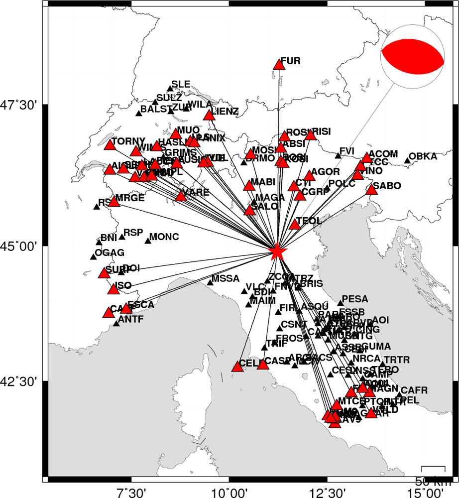
Waveform Inversion
The focal mechanism was determined using broadband seismic waveforms. The location of the event and the
and stations used for the waveform inversion are shown in the next figure.
|
|
Location of broadband stations used for waveform inversion
|
The program wvfgrd96 was used with good traces observed at short distance to determine the focal mechanism, depth and seismic moment. This technique requires a high quality signal and well determined velocity model for the Green functions. To the extent that these are the quality data, this type of mechanism should be preferred over the radiation pattern technique which requires the separate step of defining the pressure and tension quadrants and the correct strike.
The observed and predicted traces are filtered using the following gsac commands:
hp c 0.01 n 3
lp c 0.04 n 3
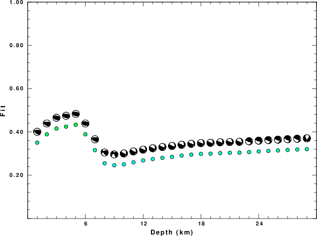
The results of this grid search from 0.5 to 19 km depth are as follow:
           DEPTH  STK   DIP  RAKE   MW    FIT
WVFGRD96    1.0   265    50    60   5.75 0.3504
WVFGRD96    2.0   270    50    70   5.81 0.3887
WVFGRD96    3.0   280    45    85   5.87 0.4155
WVFGRD96    4.0   105    45    95   5.91 0.4244
WVFGRD96    5.0   105    45    95   5.94 0.4330
WVFGRD96    6.0   105    45    95   5.95 0.3887
WVFGRD96    7.0   265    45    65   5.92 0.3158
WVFGRD96    8.0   245    55    25   5.84 0.2549
WVFGRD96    9.0   235    55   -10   5.82 0.2460
WVFGRD96   10.0    25    30    -5   5.83 0.2502
WVFGRD96   11.0    25    30    -5   5.83 0.2596
WVFGRD96   12.0    20    30    -5   5.83 0.2682
WVFGRD96   13.0    20    30    -5   5.84 0.2745
WVFGRD96   14.0    20    30    -5   5.84 0.2802
WVFGRD96   15.0    20    25    -5   5.87 0.2850
WVFGRD96   16.0    20    30    -5   5.88 0.2904
WVFGRD96   17.0    20    30    -5   5.88 0.2949
WVFGRD96   18.0    20    30    -5   5.89 0.2982
WVFGRD96   19.0    20    30    -5   5.89 0.2996
WVFGRD96   20.0    20    30    -5   5.90 0.3021
WVFGRD96   21.0    20    30    -5   5.90 0.3032
WVFGRD96   22.0    15    30   -10   5.90 0.3041
WVFGRD96   23.0   110    80    65   5.91 0.3068
WVFGRD96   24.0   110    80    65   5.91 0.3095
WVFGRD96   25.0   110    80    60   5.92 0.3121
WVFGRD96   26.0   110    80    60   5.92 0.3142
WVFGRD96   27.0   115    75    65   5.92 0.3164
WVFGRD96   28.0   115    75    65   5.93 0.3185
WVFGRD96   29.0    40    55   -35   5.99 0.3204
The best solution is
WVFGRD96 5.0 105 45 95 5.94 0.4330
The mechanism correspond to the best fit is
|
|
Figure 1. Waveform inversion focal mechanism
|
The best fit as a function of depth is given in the following figure:
|
|
Figure 2. Depth sensitivity for waveform mechanism
|
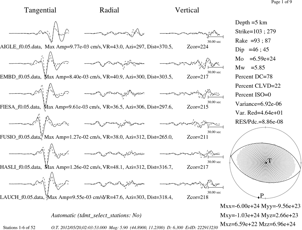
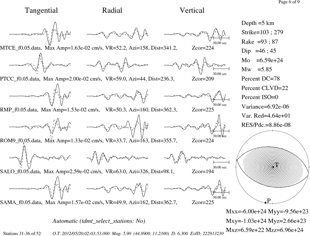
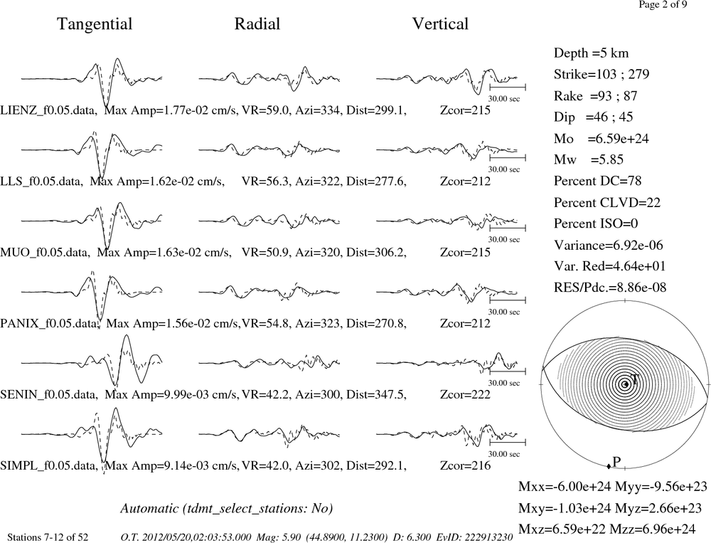
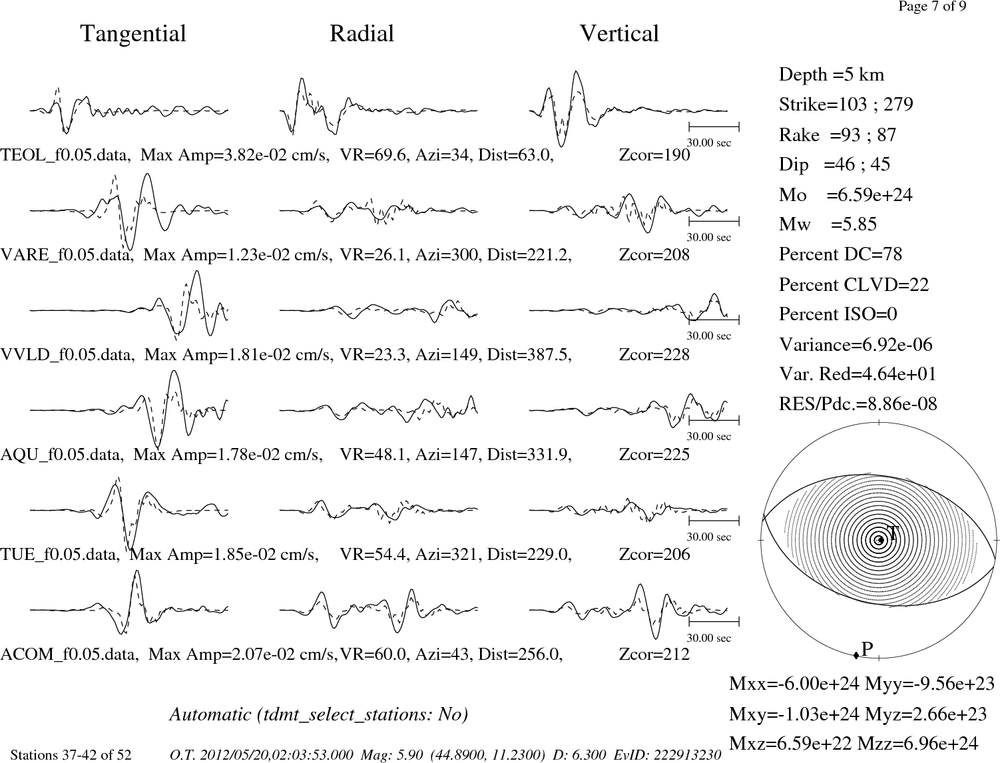
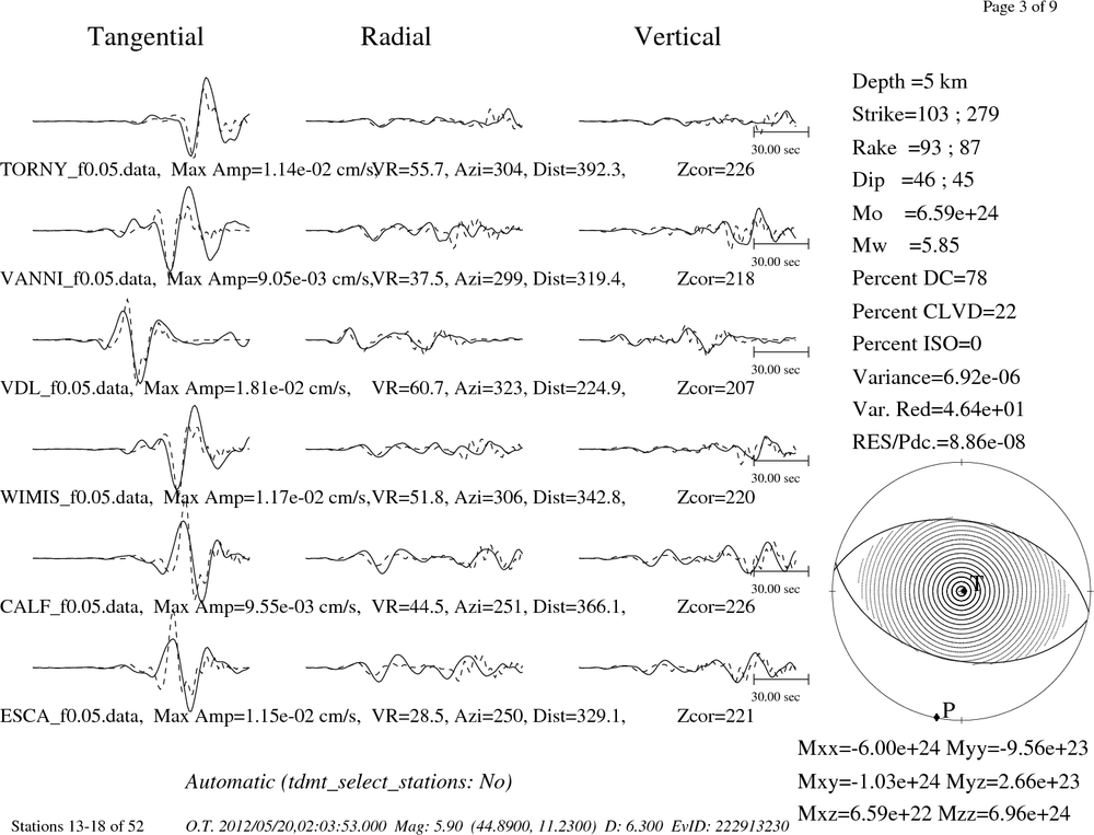
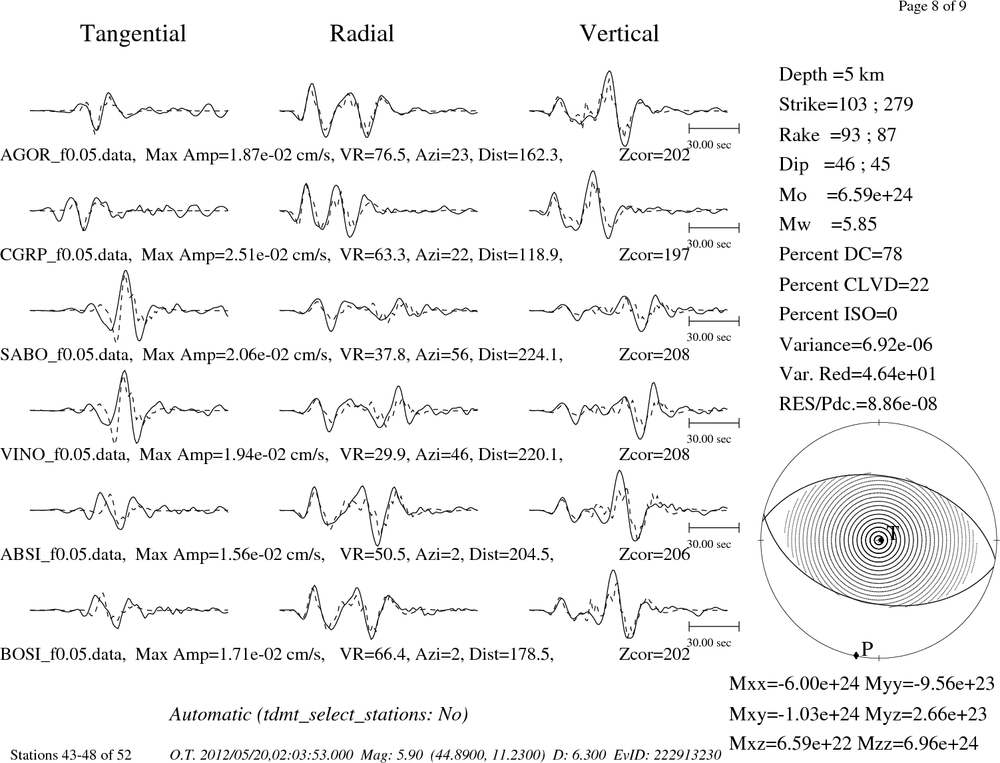
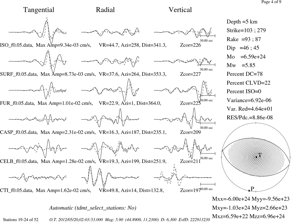
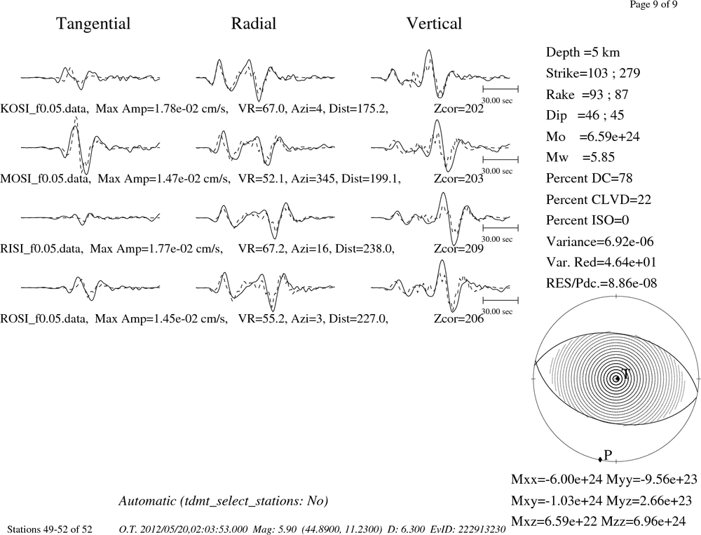
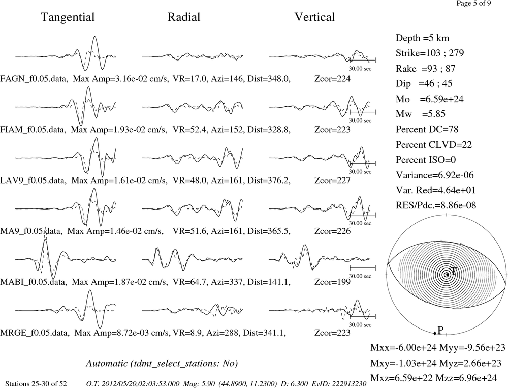
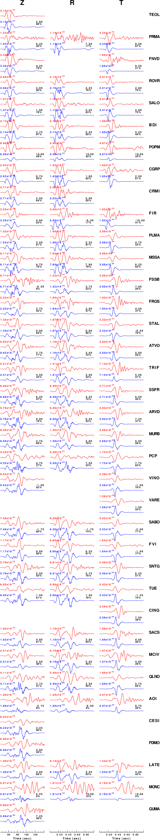
The comparison of the observed and predicted waveforms is given in the next figure. The red traces are the observed and the blue are the predicted.
Each observed-predicted component is plotted to the same scale and peak amplitudes are indicated by the numbers to the left of each trace. A pair of numbers is given in black at the right of each predicted traces. The upper number it the time shift required for maximum correlation between the observed and predicted traces. This time shift is required because the synthetics are not computed at exactly the same distance as the observed and because the velocity model used in the predictions may not be perfect.
A positive time shift indicates that the prediction is too fast and should be delayed to match the observed trace (shift to the right in this figure). A negative value indicates that the prediction is too slow. The lower number gives the percentage of variance reduction to characterize the individual goodness of fit (100% indicates a perfect fit).
The bandpass filter used in the processing and for the display was
hp c 0.01 n 3
lp c 0.04 n 3
|
|
Figure 3. Waveform comparison for selected depth
|
|
|
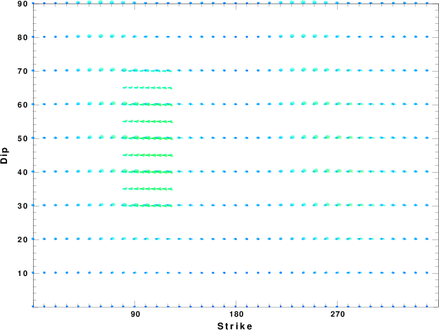
Focal mechanism sensitivity at the preferred depth. The red color indicates a very good fit to thewavefroms.
Each solution is plotted as a vector at a given value of strike and dip with the angle of the vector representing the rake angle, measured, with respect to the upward vertical (N) in the figure.
|
A check on the assumed source location is possible by looking at the time shifts between the observed and predicted traces. The time shifts for waveform matching arise for several reasons:
- The origin time and epicentral distance are incorrect
- The velocity model used for the inversion is incorrect
- The velocity model used to define the P-arrival time is not the
same as the velocity model used for the waveform inversion
(assuming that the initial trace alignment is based on the
P arrival time)
Assuming only a mislocation, the time shifts are fit to a functional form:
Time_shift = A + B cos Azimuth + C Sin Azimuth
The time shifts for this inversion lead to the next figure:
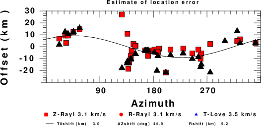
The derived shift in origin time and epicentral coordinates are given at the bottom of the figure.
Discussion
Velocity Model
The nnCIA used for the waveform synthetic seismograms and for the surface wave eigenfunctions and dispersion is as follows:
MODEL.01
C.It. A. Di Luzio et al Earth Plan Lettrs 280 (2009) 1-12 Fig 5. 7-8 MODEL/SURF3
ISOTROPIC
KGS
FLAT EARTH
1-D
CONSTANT VELOCITY
LINE08
LINE09
LINE10
LINE11
      H(KM)   VP(KM/S)   VS(KM/S) RHO(GM/CC)         QP         QS       ETAP       ETAS      FREFP      FREFS
     1.5000     3.7497     2.1436     2.2753  0.500E-02  0.100E-01   0.00       0.00       1.00       1.00
     3.0000     4.9399     2.8210     2.4858  0.500E-02  0.100E-01   0.00       0.00       1.00       1.00
     3.0000     6.0129     3.4336     2.7058  0.500E-02  0.100E-01   0.00       0.00       1.00       1.00
     7.0000     5.5516     3.1475     2.6093  0.167E-02  0.333E-02   0.00       0.00       1.00       1.00
    15.0000     5.8805     3.3583     2.6770  0.167E-02  0.333E-02   0.00       0.00       1.00       1.00
     6.0000     7.1059     4.0081     3.0002  0.167E-02  0.333E-02   0.00       0.00       1.00       1.00
     8.0000     7.1000     3.9864     3.0120  0.167E-02  0.333E-02   0.00       0.00       1.00       1.00
     0.0000     7.9000     4.4036     3.2760  0.167E-02  0.333E-02   0.00       0.00       1.00       1.00
Quality Control
Here we tabulate the reasons for not using certain digital data sets
The following stations did not have a valid response files:
DATE=Wed May 23 13:21:05 CDT 2012
Last Changed 2012/05/20