Location
2012/02/15 20:46:35 41.487 12.934 6.8 3.8 Italy
The location using elocate with a fixed depth is given in elocate.txt.
Focal Mechanism
 SLU Moment Tensor Solution
 ENS  2012/02/15 20:46:35:0  41.49   12.93   6.8 3.8 Italy

 Stations used:
   IV.CING IV.FAGN IV.FIAM IV.GUAR IV.LAV9 IV.MA9 IV.MRB1
   IV.MTCE IV.NRCA IV.OFFI IV.POFI IV.PTQR IV.SACR IV.SAMA
   IV.SGG IV.T0104 IV.TERO IV.VAGA IV.VVLD MN.AQU

 Filtering commands used:
   hp c 0.03 n 3
   lp c 0.10 n 3

 Best Fitting Double Couple
  Mo = 2.24e+21 dyne-cm
  Mw = 3.50
  Z  = 4 km
  Plane   Strike  Dip  Rake
   NP1      200    85    35
   NP2      106    55   174
  Principal Axes:
   Axis    Value   Plunge  Azimuth
    T   2.24e+21     28      69
    N   0.00e+00     55     207
    P  -2.24e+21     20     328

 Moment Tensor: (dyne-cm)
    Component   Value
       Mxx    -1.20e+21
       Mxy     1.47e+21
       Mxz    -2.82e+20
       Myy     9.77e+20
       Myz     1.24e+21
       Mzz     2.23e+20


                     --------------
                 -----------------#####
              ---   -------------#########
             ---- P ------------###########
           ------   -----------##############
          ---------------------###############
         ---------------------#################
        ---------------------############   ####
        #-------------------############# T ####
       ###------------------#############   #####
       ####----------------######################
       #####--------------#######################
       ########-----------#######################
        #########--------#######################
        ############----#######################-
         ###############-###################---
          #############-----------------------
           ############----------------------
             #########---------------------
              ########--------------------
                 ####------------------
                     --------------


 Global CMT Convention Moment Tensor:
      R          T          P
  2.23e+20  -2.82e+20  -1.24e+21
 -2.82e+20  -1.20e+21  -1.47e+21
 -1.24e+21  -1.47e+21   9.77e+20


Details of the solution is found at

http://www.eas.slu.edu/eqc/eqc_mt/MECH.IT/20120215204635/index.html
|
Preferred Solution
The preferred solution from an analysis of the surface-wave spectral amplitude radiation pattern, waveform inversion and first motion observations is
      STK = 200
      DIP = 85
     RAKE = 35
       MW = 3.50
       HS = 4.0
The waveform inversion is preferred.
Moment Tensor Comparison
The following compares this source inversion to others
| SLU |
SLU |
INGVTDMT |
 SLU Moment Tensor Solution
 ENS  2012/02/15 20:46:35:0  41.49   12.93   6.8 3.8 Italy

 Stations used:
   IV.CING IV.FAGN IV.FIAM IV.GUAR IV.LAV9 IV.MA9 IV.MRB1
   IV.MTCE IV.NRCA IV.OFFI IV.POFI IV.PTQR IV.SACR IV.SAMA
   IV.SGG IV.T0104 IV.TERO IV.VAGA IV.VVLD MN.AQU

 Filtering commands used:
   hp c 0.03 n 3
   lp c 0.10 n 3

 Best Fitting Double Couple
  Mo = 2.24e+21 dyne-cm
  Mw = 3.50
  Z  = 4 km
  Plane   Strike  Dip  Rake
   NP1      200    85    35
   NP2      106    55   174
  Principal Axes:
   Axis    Value   Plunge  Azimuth
    T   2.24e+21     28      69
    N   0.00e+00     55     207
    P  -2.24e+21     20     328

 Moment Tensor: (dyne-cm)
    Component   Value
       Mxx    -1.20e+21
       Mxy     1.47e+21
       Mxz    -2.82e+20
       Myy     9.77e+20
       Myz     1.24e+21
       Mzz     2.23e+20


                     --------------
                 -----------------#####
              ---   -------------#########
             ---- P ------------###########
           ------   -----------##############
          ---------------------###############
         ---------------------#################
        ---------------------############   ####
        #-------------------############# T ####
       ###------------------#############   #####
       ####----------------######################
       #####--------------#######################
       ########-----------#######################
        #########--------#######################
        ############----#######################-
         ###############-###################---
          #############-----------------------
           ############----------------------
             #########---------------------
              ########--------------------
                 ####------------------
                     --------------


 Global CMT Convention Moment Tensor:
      R          T          P
  2.23e+20  -2.82e+20  -1.24e+21
 -2.82e+20  -1.20e+21  -1.47e+21
 -1.24e+21  -1.47e+21   9.77e+20


Details of the solution is found at

http://www.eas.slu.edu/eqc/eqc_mt/MECH.IT/20120215204635/index.html
|
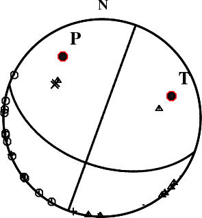
First motions and takeoff angles from an elocate run.
|
|
Waveform Inversion
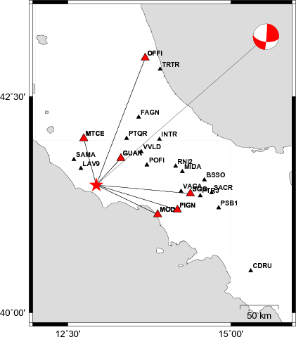
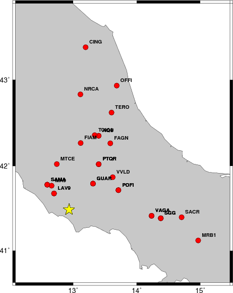
The focal mechanism was determined using broadband seismic waveforms. The location of the event and the
and stations used for the waveform inversion are shown in the next figure.
|
|
Location of broadband stations used for waveform inversion
|
The program wvfgrd96 was used with good traces observed at short distance to determine the focal mechanism, depth and seismic moment. This technique requires a high quality signal and well determined velocity model for the Green functions. To the extent that these are the quality data, this type of mechanism should be preferred over the radiation pattern technique which requires the separate step of defining the pressure and tension quadrants and the correct strike.
The observed and predicted traces are filtered using the following gsac commands:
hp c 0.03 n 3
lp c 0.10 n 3
The results of this grid search from 0.5 to 19 km depth are as follow:
           DEPTH  STK   DIP  RAKE   MW    FIT
WVFGRD96    1.0   200    90    30   3.36 0.3983
WVFGRD96    2.0    20    90   -45   3.46 0.4307
WVFGRD96    3.0   200    90    35   3.47 0.4517
WVFGRD96    4.0   200    85    35   3.50 0.4645
WVFGRD96    5.0    20    90   -40   3.56 0.4636
WVFGRD96    6.0   200    85    35   3.57 0.4566
WVFGRD96    7.0   205    75    35   3.58 0.4458
WVFGRD96    8.0   200    80    25   3.57 0.4353
WVFGRD96    9.0   200    80    25   3.58 0.4237
WVFGRD96   10.0   200    80    25   3.60 0.4109
WVFGRD96   11.0   200    80    25   3.61 0.3968
WVFGRD96   12.0   200    80    25   3.62 0.3821
WVFGRD96   13.0   200    80    25   3.63 0.3673
WVFGRD96   14.0   200    80    25   3.63 0.3522
WVFGRD96   15.0   200    80    30   3.65 0.3384
WVFGRD96   16.0   105    60   -10   3.66 0.3282
WVFGRD96   17.0   105    60   -10   3.67 0.3268
WVFGRD96   18.0   105    55   -10   3.69 0.3260
WVFGRD96   19.0   105    55    -5   3.70 0.3259
WVFGRD96   20.0   105    55    -5   3.71 0.3252
WVFGRD96   21.0   105    55   -10   3.72 0.3246
WVFGRD96   22.0   105    55   -10   3.73 0.3249
WVFGRD96   23.0   105    60   -10   3.74 0.3244
WVFGRD96   24.0   105    60   -10   3.75 0.3257
WVFGRD96   25.0   105    65   -15   3.75 0.3281
WVFGRD96   26.0   105    65   -15   3.77 0.3313
WVFGRD96   27.0   105    65   -10   3.78 0.3353
WVFGRD96   28.0   105    65   -10   3.80 0.3371
WVFGRD96   29.0   105    65   -10   3.82 0.3385
The best solution is
WVFGRD96 4.0 200 85 35 3.50 0.4645
The mechanism correspond to the best fit is
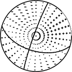
|
|
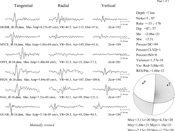
Figure 1. Waveform inversion focal mechanism
|
The best fit as a function of depth is given in the following figure:
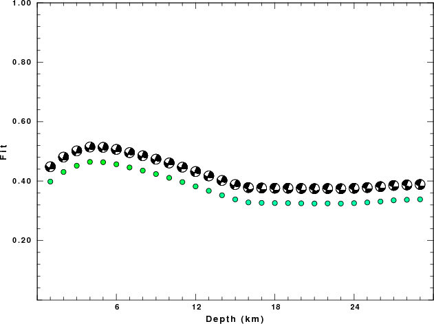
|
|
Figure 2. Depth sensitivity for waveform mechanism
|
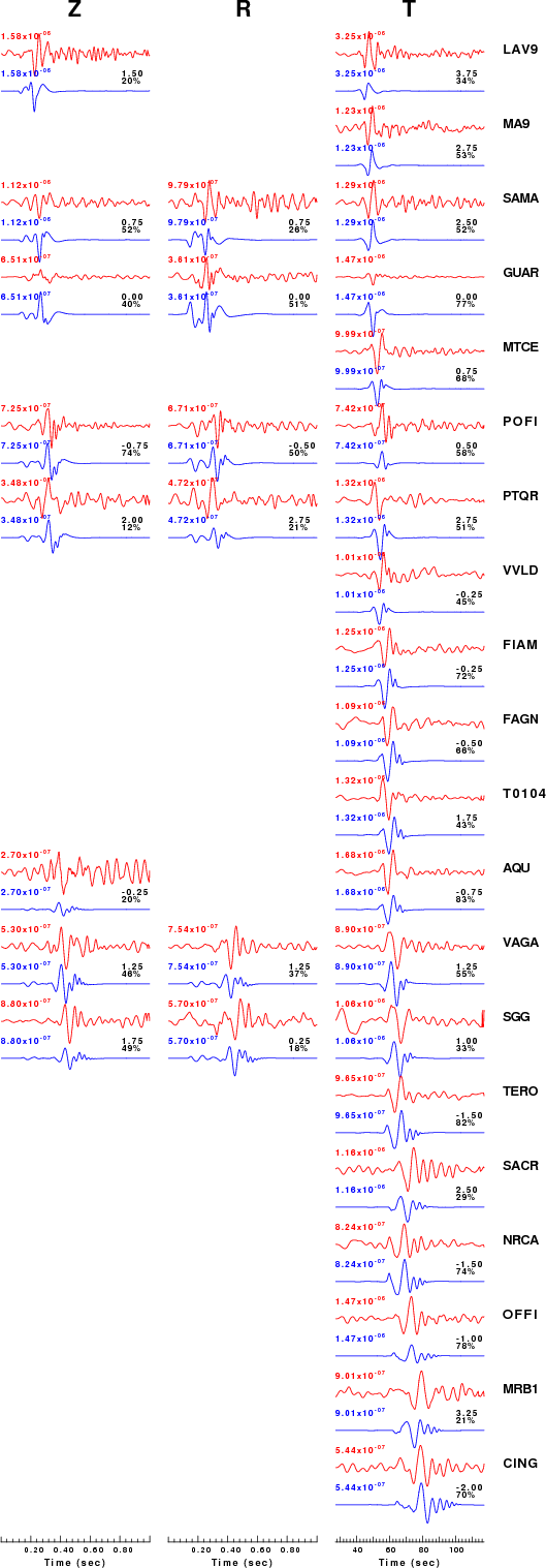
The comparison of the observed and predicted waveforms is given in the next figure. The red traces are the observed and the blue are the predicted.
Each observed-predicted component is plotted to the same scale and peak amplitudes are indicated by the numbers to the left of each trace. A pair of numbers is given in black at the right of each predicted traces. The upper number it the time shift required for maximum correlation between the observed and predicted traces. This time shift is required because the synthetics are not computed at exactly the same distance as the observed and because the velocity model used in the predictions may not be perfect.
A positive time shift indicates that the prediction is too fast and should be delayed to match the observed trace (shift to the right in this figure). A negative value indicates that the prediction is too slow. The lower number gives the percentage of variance reduction to characterize the individual goodness of fit (100% indicates a perfect fit).
The bandpass filter used in the processing and for the display was
hp c 0.03 n 3
lp c 0.10 n 3
|
|
Figure 3. Waveform comparison for selected depth
|
|
|
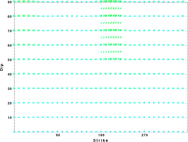
Focal mechanism sensitivity at the preferred depth. The red color indicates a very good fit to thewavefroms.
Each solution is plotted as a vector at a given value of strike and dip with the angle of the vector representing the rake angle, measured, with respect to the upward vertical (N) in the figure.
|
A check on the assumed source location is possible by looking at the time shifts between the observed and predicted traces. The time shifts for waveform matching arise for several reasons:
- The origin time and epicentral distance are incorrect
- The velocity model used for the inversion is incorrect
- The velocity model used to define the P-arrival time is not the
same as the velocity model used for the waveform inversion
(assuming that the initial trace alignment is based on the
P arrival time)
Assuming only a mislocation, the time shifts are fit to a functional form:
Time_shift = A + B cos Azimuth + C Sin Azimuth
The time shifts for this inversion lead to the next figure:
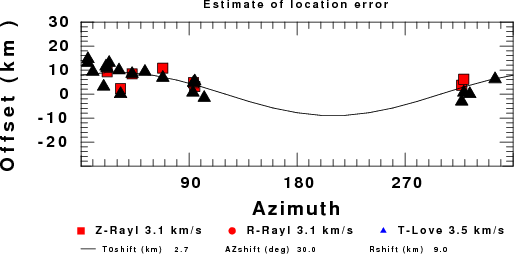
The derived shift in origin time and epicentral coordinates are given at the bottom of the figure.
Discussion
Velocity Model
The nnCIA used for the waveform synthetic seismograms and for the surface wave eigenfunctions and dispersion is as follows:
MODEL.01
C.It. A. Di Luzio et al Earth Plan Lettrs 280 (2009) 1-12 Fig 5. 7-8 MODEL/SURF3
ISOTROPIC
KGS
FLAT EARTH
1-D
CONSTANT VELOCITY
LINE08
LINE09
LINE10
LINE11
      H(KM)   VP(KM/S)   VS(KM/S) RHO(GM/CC)         QP         QS       ETAP       ETAS      FREFP      FREFS
     1.5000     3.7497     2.1436     2.2753  0.500E-02  0.100E-01   0.00       0.00       1.00       1.00
     3.0000     4.9399     2.8210     2.4858  0.500E-02  0.100E-01   0.00       0.00       1.00       1.00
     3.0000     6.0129     3.4336     2.7058  0.500E-02  0.100E-01   0.00       0.00       1.00       1.00
     7.0000     5.5516     3.1475     2.6093  0.167E-02  0.333E-02   0.00       0.00       1.00       1.00
    15.0000     5.8805     3.3583     2.6770  0.167E-02  0.333E-02   0.00       0.00       1.00       1.00
     6.0000     7.1059     4.0081     3.0002  0.167E-02  0.333E-02   0.00       0.00       1.00       1.00
     8.0000     7.1000     3.9864     3.0120  0.167E-02  0.333E-02   0.00       0.00       1.00       1.00
     0.0000     7.9000     4.4036     3.2760  0.167E-02  0.333E-02   0.00       0.00       1.00       1.00
Quality Control
Here we tabulate the reasons for not using certain digital data sets
The following stations did not have a valid response files:
DATE=Fri Feb 17 11:51:36 CST 2012
Last Changed 2012/02/15