Location
2012/01/27 14:53:13 44.483 10.033 5.4 60.8 Italy
Arrival Times (from USGS)
Arrival time list
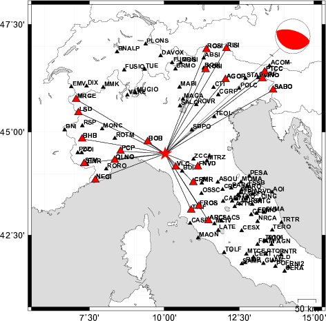
Felt Map
USGS Felt map for this earthquake
USGS Felt reports page for
Focal Mechanism
 SLU Moment Tensor Solution
 ENS  2012/01/27 14:53:13:0  44.48   10.03   5.4 60.8 Italy

 Stations used:
   GU.BHB GU.FINB GU.NEGI GU.PCP GU.RORO GU.RSP GU.STV GU.TRAV
   IV.BOB IV.CASP IV.CRMI IV.DOI IV.FIR IV.FNVD IV.FROS
   IV.MABI IV.MCIV IV.MSSA IV.MTRZ IV.PARC IV.PIEI IV.PLMA
   IV.PRMA IV.QLNO IV.ROVR IV.TRIF MN.TUE MN.VLC NI.CGRP

 Filtering commands used:
   hp c 0.02 n 3
   lp c 0.06 n 3

 Best Fitting Double Couple
  Mo = 4.12e+23 dyne-cm
  Mw = 5.01
  Z  = 54 km
  Plane   Strike  Dip  Rake
   NP1      294    65    88
   NP2      120    25    95
  Principal Axes:
   Axis    Value   Plunge  Azimuth
    T   4.12e+23     70     200
    N   0.00e+00      2     295
    P  -4.12e+23     20      26

 Moment Tensor: (dyne-cm)
    Component   Value
       Mxx    -2.49e+23
       Mxy    -1.29e+23
       Mxz    -2.45e+23
       Myy    -6.55e+22
       Myz    -1.04e+23
       Mzz     3.14e+23


                     --------------
                 -----------------   --
              -------------------- P -----
             ---------------------   ------
           ----------------------------------
          ------------------------------------
         -#############------------------------
        -####################-------------------
        -########################---------------
       --###########################-------------
       ---#############################----------
       ---###############################--------
       ----##############   ###############------
        ---############## T #################---
        -----############   ##################--
         -----#################################
          ------##############################
           -------##########################-
             -------######################-
              -----------############-----
                 ----------------------
                     --------------


 Global CMT Convention Moment Tensor:
      R          T          P
  3.14e+23  -2.45e+23   1.04e+23
 -2.45e+23  -2.49e+23   1.29e+23
  1.04e+23   1.29e+23  -6.55e+22


Details of the solution is found at

http://www.eas.slu.edu/eqc/eqc_mt/MECH.IT/20120127145313/index.html
|
Preferred Solution
The preferred solution from an analysis of the surface-wave spectral amplitude radiation pattern, waveform inversion and first motion observations is
      STK = 120
      DIP = 25
     RAKE = 95
       MW = 5.01
       HS = 54.0
The WUS model was used sinc ethe lower crust of nnCIA is not well defined and since I did not have Green functions for the deepter depths requried for this event.
Moment Tensor Comparison
The following compares this source inversion to others
| SLU |
INGVTDMT |
 SLU Moment Tensor Solution
 ENS  2012/01/27 14:53:13:0  44.48   10.03   5.4 60.8 Italy

 Stations used:
   GU.BHB GU.FINB GU.NEGI GU.PCP GU.RORO GU.RSP GU.STV GU.TRAV
   IV.BOB IV.CASP IV.CRMI IV.DOI IV.FIR IV.FNVD IV.FROS
   IV.MABI IV.MCIV IV.MSSA IV.MTRZ IV.PARC IV.PIEI IV.PLMA
   IV.PRMA IV.QLNO IV.ROVR IV.TRIF MN.TUE MN.VLC NI.CGRP

 Filtering commands used:
   hp c 0.02 n 3
   lp c 0.06 n 3

 Best Fitting Double Couple
  Mo = 4.12e+23 dyne-cm
  Mw = 5.01
  Z  = 54 km
  Plane   Strike  Dip  Rake
   NP1      294    65    88
   NP2      120    25    95
  Principal Axes:
   Axis    Value   Plunge  Azimuth
    T   4.12e+23     70     200
    N   0.00e+00      2     295
    P  -4.12e+23     20      26

 Moment Tensor: (dyne-cm)
    Component   Value
       Mxx    -2.49e+23
       Mxy    -1.29e+23
       Mxz    -2.45e+23
       Myy    -6.55e+22
       Myz    -1.04e+23
       Mzz     3.14e+23


                     --------------
                 -----------------   --
              -------------------- P -----
             ---------------------   ------
           ----------------------------------
          ------------------------------------
         -#############------------------------
        -####################-------------------
        -########################---------------
       --###########################-------------
       ---#############################----------
       ---###############################--------
       ----##############   ###############------
        ---############## T #################---
        -----############   ##################--
         -----#################################
          ------##############################
           -------##########################-
             -------######################-
              -----------############-----
                 ----------------------
                     --------------


 Global CMT Convention Moment Tensor:
      R          T          P
  3.14e+23  -2.45e+23   1.04e+23
 -2.45e+23  -2.49e+23   1.29e+23
  1.04e+23   1.29e+23  -6.55e+22


Details of the solution is found at

http://www.eas.slu.edu/eqc/eqc_mt/MECH.IT/20120127145313/index.html
|
|
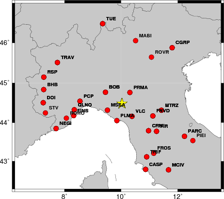
Waveform Inversion
The focal mechanism was determined using broadband seismic waveforms. The location of the event and the
and stations used for the waveform inversion are shown in the next figure.
|
|
Location of broadband stations used for waveform inversion
|
The program wvfgrd96 was used with good traces observed at short distance to determine the focal mechanism, depth and seismic moment. This technique requires a high quality signal and well determined velocity model for the Green functions. To the extent that these are the quality data, this type of mechanism should be preferred over the radiation pattern technique which requires the separate step of defining the pressure and tension quadrants and the correct strike.
The observed and predicted traces are filtered using the following gsac commands:
hp c 0.02 n 3
lp c 0.06 n 3
The results of this grid search from 0.5 to 19 km depth are as follow:
           DEPTH  STK   DIP  RAKE   MW    FIT
WVFGRD96    1.0   295    40   -90   4.26 0.1545
WVFGRD96    2.0   295    40   -90   4.38 0.1999
WVFGRD96    3.0   120    65   -85   4.46 0.2048
WVFGRD96    4.0   290    25   -95   4.48 0.2157
WVFGRD96    5.0   290    25  -100   4.48 0.2238
WVFGRD96    6.0   110    70   -90   4.48 0.2373
WVFGRD96    7.0   115    70   -90   4.49 0.2499
WVFGRD96    8.0   290    20   -95   4.56 0.2664
WVFGRD96    9.0   285    20  -100   4.56 0.2764
WVFGRD96   10.0   285    20  -100   4.56 0.2838
WVFGRD96   11.0   120    70   -80   4.56 0.2898
WVFGRD96   12.0   125    70   -75   4.56 0.2982
WVFGRD96   13.0   125    70   -75   4.57 0.3058
WVFGRD96   14.0   125    70   -75   4.57 0.3127
WVFGRD96   15.0   125    70   -75   4.58 0.3188
WVFGRD96   16.0   125    75   -70   4.58 0.3250
WVFGRD96   17.0   125    75   -70   4.59 0.3311
WVFGRD96   18.0   125    75   -70   4.60 0.3363
WVFGRD96   19.0   125    75   -70   4.61 0.3393
WVFGRD96   20.0   125    75   -70   4.61 0.3424
WVFGRD96   21.0   125    75   -70   4.63 0.3485
WVFGRD96   22.0   125    75   -70   4.64 0.3505
WVFGRD96   23.0   125    75   -70   4.64 0.3499
WVFGRD96   24.0   130    80   -65   4.65 0.3518
WVFGRD96   25.0   130    80   -65   4.66 0.3527
WVFGRD96   26.0   130    80   -65   4.66 0.3528
WVFGRD96   27.0   130    80   -70   4.67 0.3530
WVFGRD96   28.0    40    25    20   4.67 0.3534
WVFGRD96   29.0    45    25    25   4.67 0.3588
WVFGRD96   30.0   130    10   105   4.69 0.3672
WVFGRD96   31.0   295    80    85   4.70 0.3756
WVFGRD96   32.0   295    80    85   4.71 0.3834
WVFGRD96   33.0   295    80    85   4.71 0.3911
WVFGRD96   34.0   295    80    85   4.72 0.3979
WVFGRD96   35.0   295    75    85   4.73 0.4058
WVFGRD96   36.0   295    75    85   4.74 0.4128
WVFGRD96   37.0   125    15   100   4.74 0.4184
WVFGRD96   38.0   295    70    85   4.76 0.4259
WVFGRD96   39.0   295    65    85   4.78 0.4341
WVFGRD96   40.0   125    25   100   4.90 0.4289
WVFGRD96   41.0   125    25   100   4.91 0.4389
WVFGRD96   42.0   120    25    95   4.92 0.4480
WVFGRD96   43.0   295    65    85   4.93 0.4566
WVFGRD96   44.0   120    25    95   4.94 0.4642
WVFGRD96   45.0   120    25    95   4.95 0.4715
WVFGRD96   46.0   295    65    85   4.96 0.4775
WVFGRD96   47.0   295    65    85   4.97 0.4835
WVFGRD96   48.0   120    25    95   4.97 0.4883
WVFGRD96   49.0   120    25    95   4.98 0.4923
WVFGRD96   50.0   295    65    85   4.99 0.4956
WVFGRD96   51.0   295    65    85   4.99 0.4976
WVFGRD96   52.0   120    25    95   5.00 0.4999
WVFGRD96   53.0   120    25    95   5.00 0.5001
WVFGRD96   54.0   120    25    95   5.01 0.5007
WVFGRD96   55.0   120    25    95   5.01 0.4999
WVFGRD96   56.0   295    65    85   5.02 0.4982
WVFGRD96   57.0   295    65    85   5.02 0.4961
WVFGRD96   58.0   295    65    85   5.02 0.4932
WVFGRD96   59.0   295    65    85   5.03 0.4905
WVFGRD96   60.0   295    65    85   5.03 0.4863
WVFGRD96   61.0   295    65    85   5.03 0.4821
WVFGRD96   62.0   295    65    85   5.03 0.4774
WVFGRD96   63.0   295    65    85   5.03 0.4718
WVFGRD96   64.0   295    65    85   5.03 0.4665
WVFGRD96   65.0   290    65    90   5.03 0.4606
WVFGRD96   66.0   290    65    90   5.03 0.4547
WVFGRD96   67.0   290    65    90   5.03 0.4486
WVFGRD96   68.0   290    65    90   5.03 0.4425
WVFGRD96   69.0   290    65    85   5.03 0.4356
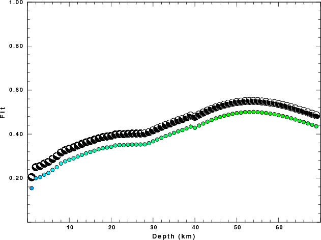
The best solution is
WVFGRD96 54.0 120 25 95 5.01 0.5007
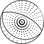
The mechanism correspond to the best fit is
|
|
Figure 1. Waveform inversion focal mechanism
|
The best fit as a function of depth is given in the following figure:
|
|
Figure 2. Depth sensitivity for waveform mechanism
|
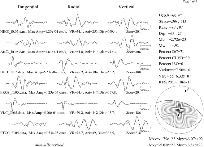
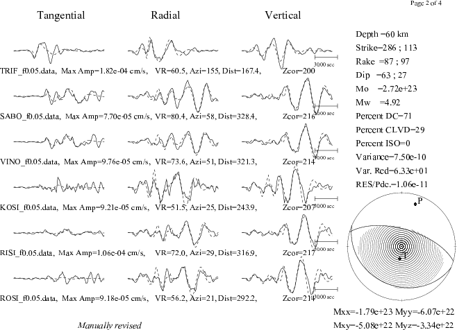
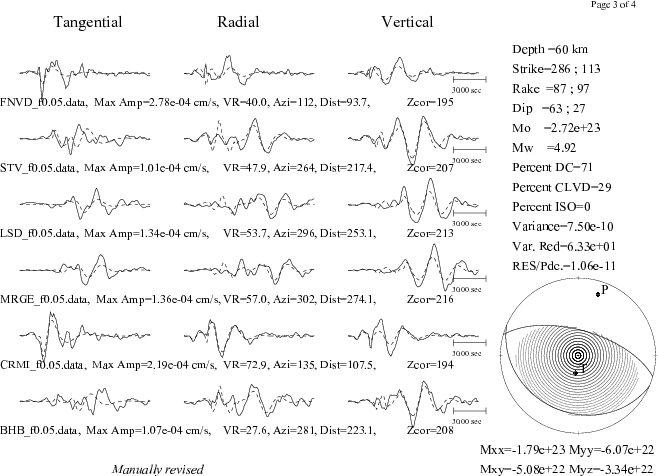
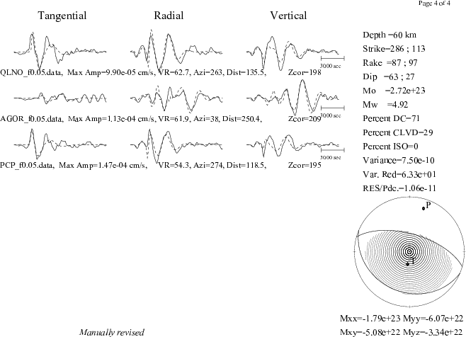
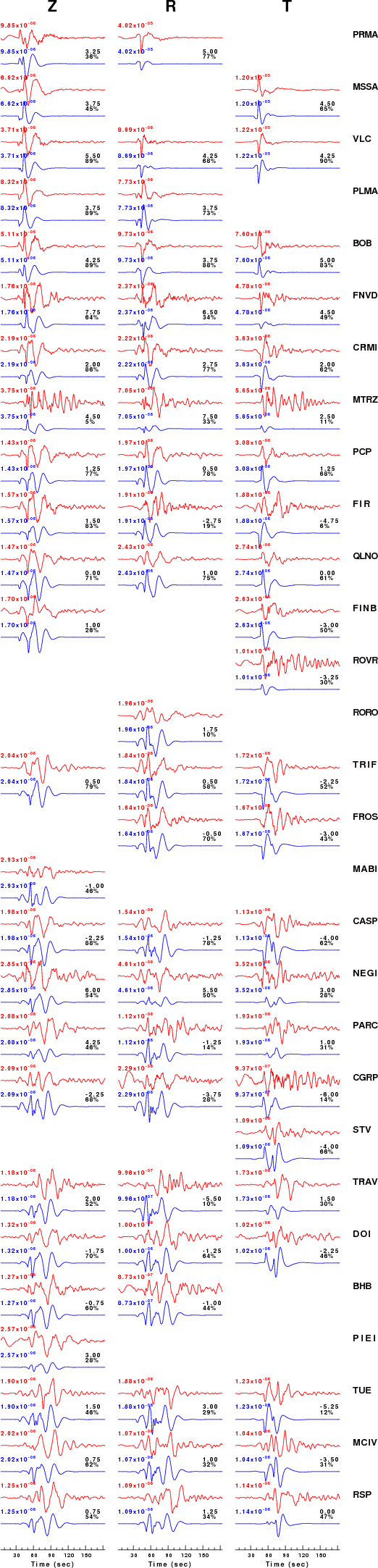
The comparison of the observed and predicted waveforms is given in the next figure. The red traces are the observed and the blue are the predicted.
Each observed-predicted component is plotted to the same scale and peak amplitudes are indicated by the numbers to the left of each trace. A pair of numbers is given in black at the right of each predicted traces. The upper number it the time shift required for maximum correlation between the observed and predicted traces. This time shift is required because the synthetics are not computed at exactly the same distance as the observed and because the velocity model used in the predictions may not be perfect.
A positive time shift indicates that the prediction is too fast and should be delayed to match the observed trace (shift to the right in this figure). A negative value indicates that the prediction is too slow. The lower number gives the percentage of variance reduction to characterize the individual goodness of fit (100% indicates a perfect fit).
The bandpass filter used in the processing and for the display was
hp c 0.02 n 3
lp c 0.06 n 3
|
|
Figure 3. Waveform comparison for selected depth
|
|
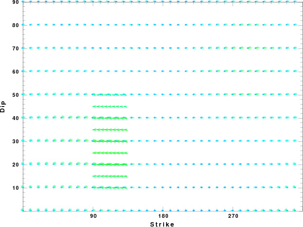
|
Focal mechanism sensitivity at the preferred depth. The red color indicates a very good fit to thewavefroms.
Each solution is plotted as a vector at a given value of strike and dip with the angle of the vector representing the rake angle, measured, with respect to the upward vertical (N) in the figure.
|
A check on the assumed source location is possible by looking at the time shifts between the observed and predicted traces. The time shifts for waveform matching arise for several reasons:
- The origin time and epicentral distance are incorrect
- The velocity model used for the inversion is incorrect
- The velocity model used to define the P-arrival time is not the
same as the velocity model used for the waveform inversion
(assuming that the initial trace alignment is based on the
P arrival time)
Assuming only a mislocation, the time shifts are fit to a functional form:
Time_shift = A + B cos Azimuth + C Sin Azimuth
The time shifts for this inversion lead to the next figure:
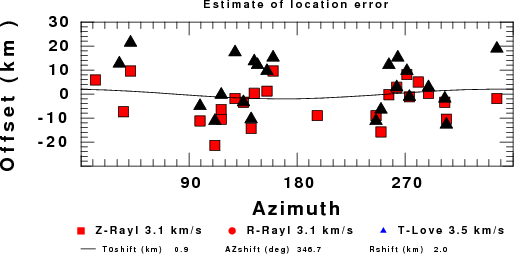
The derived shift in origin time and epicentral coordinates are given at the bottom of the figure.
Discussion
Velocity Model
The WUS used for the waveform synthetic seismograms and for the surface wave eigenfunctions and dispersion is as follows:
MODEL.01
Model after     8 iterations
ISOTROPIC
KGS
FLAT EARTH
1-D
CONSTANT VELOCITY
LINE08
LINE09
LINE10
LINE11
      H(KM)   VP(KM/S)   VS(KM/S) RHO(GM/CC)         QP         QS       ETAP       ETAS      FREFP      FREFS
     1.9000     3.4065     2.0089     2.2150  0.302E-02  0.679E-02   0.00       0.00       1.00       1.00
     6.1000     5.5445     3.2953     2.6089  0.349E-02  0.784E-02   0.00       0.00       1.00       1.00
    13.0000     6.2708     3.7396     2.7812  0.212E-02  0.476E-02   0.00       0.00       1.00       1.00
    19.0000     6.4075     3.7680     2.8223  0.111E-02  0.249E-02   0.00       0.00       1.00       1.00
     0.0000     7.9000     4.6200     3.2760  0.164E-10  0.370E-10   0.00       0.00       1.00       1.00
Quality Control
Here we tabulate the reasons for not using certain digital data sets
The following stations did not have a valid response files:
DATE=Thu Feb 16 11:22:57 CST 2012
Last Changed 2012/01/27