Location
INGV Automatic Location
2011/06/19 14:35:34 44.09 10.76 15. 3.6 Italy
Focal Mechanism
USGS/SLU Moment Tensor Solution
ENS 2011/06/19 14:35:34:0 44.09 10.76 15.0 3.6 Italy
Stations used:
GU.MAIM GU.SC2M IV.ARCI IV.ASQU IV.ATPC IV.BDI IV.BOB
IV.CAFI IV.CASP IV.CRE IV.CRMI IV.FNVD IV.FROS IV.GROG
IV.MSSA IV.PARC IV.PLMA IV.PRMA IV.SASS MN.VLC
Filtering commands used:
hp c 0.02 n 3
lp c 0.10 n 3
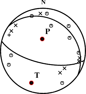
Best Fitting Double Couple
Mo = 4.79e+21 dyne-cm
Mw = 3.72
Z = 8 km
Plane Strike Dip Rake
NP1 103 67 -99
NP2 305 25 -70
Principal Axes:
Axis Value Plunge Azimuth
T 4.79e+21 21 200
N 0.00e+00 8 107
P -4.79e+21 67 356
Moment Tensor: (dyne-cm)
Component Value
Mxx 2.96e+21
Mxy 1.38e+21
Mxz -3.22e+21
Myy 4.83e+20
Myz -4.43e+20
Mzz -3.45e+21
##############
######################
###---------------##########
#----------------------#######
---------------------------#######
------------------------------######
----------------- -------------#####
------------------ P --------------#####
------------------ ---------------####
##------------------------------------####
#####----------------------------------###
#######--------------------------------###
###########----------------------------###
##############------------------------##
######################-------------###--
#####################################-
####################################
##################################
######## ###################
####### T ##################
#### ###############
##############
Global CMT Convention Moment Tensor:
R T P
-3.45e+21 -3.22e+21 4.43e+20
-3.22e+21 2.96e+21 -1.38e+21
4.43e+20 -1.38e+21 4.83e+20
Details of the solution is found at
http://www.eas.slu.edu/eqc/eqc_mt/MECH.IT/20110619143534/index.html
|
Preferred Solution
The preferred solution from an analysis of the surface-wave spectral amplitude radiation pattern, waveform inversion and first motion observations is
      STK = 305
      DIP = 25
     RAKE = -70
       MW = 3.72
       HS = 8.0
The waveform inversion is preferred.
Moment Tensor Comparison
The following compares this source inversion to others
| SLU |
SLU |
 USGS/SLU Moment Tensor Solution
 ENS  2011/06/19 14:35:34:0  44.09   10.76  15.0 3.6 Italy

 Stations used:
   GU.MAIM GU.SC2M IV.ARCI IV.ASQU IV.ATPC IV.BDI IV.BOB
   IV.CAFI IV.CASP IV.CRE IV.CRMI IV.FNVD IV.FROS IV.GROG
   IV.MSSA IV.PARC IV.PLMA IV.PRMA IV.SASS MN.VLC

 Filtering commands used:
   hp c 0.02 n 3
   lp c 0.10 n 3

 Best Fitting Double Couple
  Mo = 4.79e+21 dyne-cm
  Mw = 3.72
  Z  = 8 km
  Plane   Strike  Dip  Rake
   NP1      103    67   -99
   NP2      305    25   -70
  Principal Axes:
   Axis    Value   Plunge  Azimuth
    T   4.79e+21     21     200
    N   0.00e+00      8     107
    P  -4.79e+21     67     356

 Moment Tensor: (dyne-cm)
    Component   Value
       Mxx     2.96e+21
       Mxy     1.38e+21
       Mxz    -3.22e+21
       Myy     4.83e+20
       Myz    -4.43e+20
       Mzz    -3.45e+21


                     ##############
                 ######################
              ###---------------##########
             #----------------------#######
           ---------------------------#######
          ------------------------------######
         -----------------   -------------#####
        ------------------ P --------------#####
        ------------------   ---------------####
       ##------------------------------------####
       #####----------------------------------###
       #######--------------------------------###
       ###########----------------------------###
        ##############------------------------##
        ######################-------------###--
         #####################################-
          ####################################
           ##################################
             ########   ###################
              ####### T ##################
                 ####   ###############
                     ##############


 Global CMT Convention Moment Tensor:
      R          T          P
 -3.45e+21  -3.22e+21   4.43e+20
 -3.22e+21   2.96e+21  -1.38e+21
  4.43e+20  -1.38e+21   4.83e+20


Details of the solution is found at

http://www.eas.slu.edu/eqc/eqc_mt/MECH.IT/20110619143534/index.html
|
First motions and takeoff angles from an elocate run.
|
Waveform Inversion
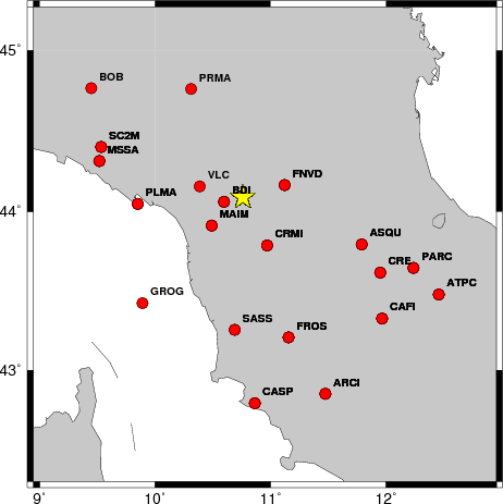
The focal mechanism was determined using broadband seismic waveforms. The location of the event and the
and stations used for the waveform inversion are shown in the next figure.
|
|
Location of broadband stations used for waveform inversion
|
The program wvfgrd96 was used with good traces observed at short distance to determine the focal mechanism, depth and seismic moment. This technique requires a high quality signal and well determined velocity model for the Green functions. To the extent that these are the quality data, this type of mechanism should be preferred over the radiation pattern technique which requires the separate step of defining the pressure and tension quadrants and the correct strike.
The observed and predicted traces are filtered using the following gsac commands:
hp c 0.02 n 3
lp c 0.10 n 3
The results of this grid search from 0.5 to 19 km depth are as follow:
           DEPTH  STK   DIP  RAKE   MW    FIT
WVFGRD96    1.0    95    50   -85   3.52 0.3449
WVFGRD96    2.0   100    70   -85   3.62 0.3104
WVFGRD96    3.0   310    10   -60   3.63 0.3973
WVFGRD96    4.0   300    15   -70   3.62 0.4608
WVFGRD96    5.0   300    15   -70   3.74 0.5118
WVFGRD96    6.0   300    20   -70   3.75 0.5535
WVFGRD96    7.0   300    20   -70   3.75 0.5734
WVFGRD96    8.0   305    25   -70   3.72 0.5814
WVFGRD96    9.0   305    25   -70   3.72 0.5799
WVFGRD96   10.0   310    25   -65   3.73 0.5724
WVFGRD96   11.0   320    30   -55   3.74 0.5613
WVFGRD96   12.0   315    25   -55   3.74 0.5475
WVFGRD96   13.0   315    25   -55   3.74 0.5316
WVFGRD96   14.0   320    25   -50   3.75 0.5137
WVFGRD96   15.0   315    25   -55   3.79 0.4981
WVFGRD96   16.0   320    25   -50   3.79 0.4780
WVFGRD96   17.0   315    20   -55   3.80 0.4592
WVFGRD96   18.0    95    55    45   3.81 0.4439
WVFGRD96   19.0    95    55    45   3.82 0.4280
WVFGRD96   20.0   100    50    45   3.82 0.4109
WVFGRD96   21.0   305    20   -70   3.82 0.3959
WVFGRD96   22.0   305    20   -70   3.83 0.3828
WVFGRD96   23.0   305    20   -70   3.83 0.3699
WVFGRD96   24.0   315    25   -60   3.84 0.3594
WVFGRD96   25.0   315    25   -60   3.84 0.3479
WVFGRD96   26.0   310    25   -65   3.84 0.3348
WVFGRD96   27.0   325    30   -55   3.84 0.3226
WVFGRD96   28.0   315    30   -60   3.85 0.3107
WVFGRD96   29.0   325    35   -55   3.85 0.2997
The best solution is
WVFGRD96 8.0 305 25 -70 3.72 0.5814
The mechanism correspond to the best fit is
|
|
Figure 1. Waveform inversion focal mechanism
|
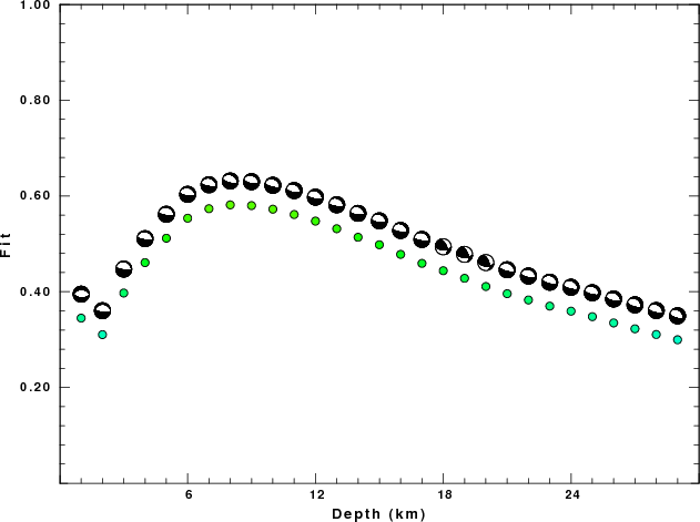
The best fit as a function of depth is given in the following figure:
|
|
Figure 2. Depth sensitivity for waveform mechanism
|
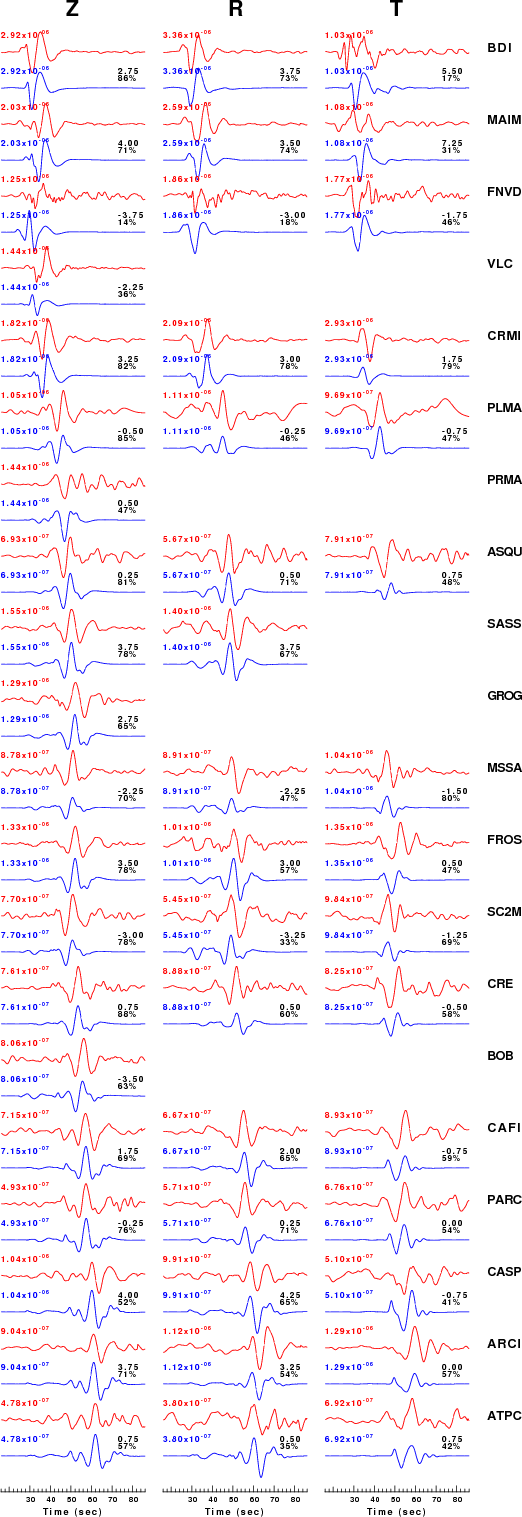
The comparison of the observed and predicted waveforms is given in the next figure. The red traces are the observed and the blue are the predicted.
Each observed-predicted component is plotted to the same scale and peak amplitudes are indicated by the numbers to the left of each trace. A pair of numbers is given in black at the right of each predicted traces. The upper number it the time shift required for maximum correlation between the observed and predicted traces. This time shift is required because the synthetics are not computed at exactly the same distance as the observed and because the velocity model used in the predictions may not be perfect.
A positive time shift indicates that the prediction is too fast and should be delayed to match the observed trace (shift to the right in this figure). A negative value indicates that the prediction is too slow. The lower number gives the percentage of variance reduction to characterize the individual goodness of fit (100% indicates a perfect fit).
The bandpass filter used in the processing and for the display was
hp c 0.02 n 3
lp c 0.10 n 3
|
|
Figure 3. Waveform comparison for selected depth
|
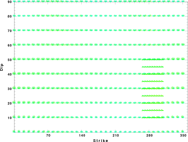
|
|
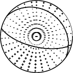
Focal mechanism sensitivity at the preferred depth. The red color indicates a very good fit to thewavefroms.
Each solution is plotted as a vector at a given value of strike and dip with the angle of the vector representing the rake angle, measured, with respect to the upward vertical (N) in the figure.
|
A check on the assumed source location is possible by looking at the time shifts between the observed and predicted traces. The time shifts for waveform matching arise for several reasons:
- The origin time and epicentral distance are incorrect
- The velocity model used for the inversion is incorrect
- The velocity model used to define the P-arrival time is not the
same as the velocity model used for the waveform inversion
(assuming that the initial trace alignment is based on the
P arrival time)
Assuming only a mislocation, the time shifts are fit to a functional form:
Time_shift = A + B cos Azimuth + C Sin Azimuth
The time shifts for this inversion lead to the next figure:
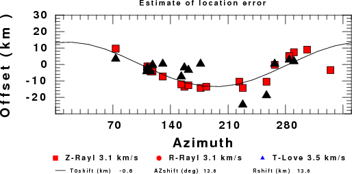
The derived shift in origin time and epicentral coordinates are given at the bottom of the figure.
Elocate Location
This event had a very good waveform fit. However the analysis of the time shifts required to fit the waveform, indicated that the waveforms would be better fit if the location was moved about 13 km in a direction of 14 degrees from the INGV location. The origin time shift of 0.5 sec earlier is on the order of the Greens function sampling and does not suggest a difference in origin time. Note that the actual shift will be less since the assumed velocities are too high for the region - average velocities of about 2.9 km/s for Love and 2.6 km/sec for Rayleigh would be more appropriate. Using these velocities would suggest a shift of about 11 km.
The program elocate was uses after manually picking arrival times. The nnCIA velocity model, listed below, was used for the location. The detailed processing results are given in the file
elocate.txt. The elocate solution is
      RMS Error        :               0.112              sec
      Travel_Time_Table:          nnCIA
      Latitude         :             44.1397 +-    0.0085 N         0.9449 km
      Longitude        :             10.8199 +-    0.0086 E         0.6829 km
      Depth            :               14.55 +-      2.17 km
      Epoch Time       :      1308494134.000 +-      0.15 sec
      Event Time       :  20110619143534.000 +-      0.15 sec
      Event (OCAL)     :  2011 06 19 14 35 34 000
      HYPO71 Quality   :                  CB
      Gap              :                  98              deg
This solution is 7.3 km from the INGV automatic solution in a direction 41 degrees east of north. This movement is similar to that suggested by the waveform analysis.
This relocation supports the suggestion that the initial INGV solution is biased slightly. If we had used these source coordinates instead fo the INGV automatic solution, the amplitude of the azimuthal delay plot would have been reduced.
To demonstrate the improvement, the elocate coordinates were used for the location and the source inversion was rrun again. The best solution had the parameters
           H(km)  STK   DIP  RAKE    Mw    Fit
WVFGRD96    8.0   110    65   -95   3.75 0.6368
or
            8.0   302    25   -79
This goodness of fit is better than that of the original grid search above
which had the solution
           H(km)  STK   DIP  RAKE    Mw    Fit
WVFGRD96    8.0   305    25   -70   3.72 0.5814
The plot based on the time shifts required for the elocate soution is shown in the next figure.
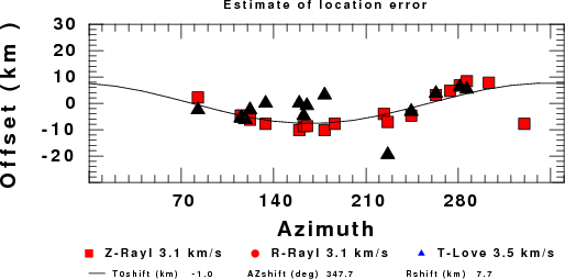
The derived shift in origin time and epicentral coordinates are given at the bottom of the figure.
As expected, the amplitude of the sine function is smaller. However the waveform shift continue to require a location even farther north.
The analysis of the waveform time shifts indicate the need for a careful relocation of the earthquake. The exact location of the event cannot be determined here because of the lack of complete azimuthal coverage for first arrival location and for source inversion. The simplified analysis performed here used a 1-D velocity model for location and for source inversion.
Discussion
Velocity Model
The nnCIA used for the waveform synthetic seismograms and for the surface wave eigenfunctions and dispersion is as follows:
MODEL.01
C.It. A. Di Luzio et al Earth Plan Lettrs 280 (2009) 1-12 Fig 5. 7-8 MODEL/SURF3
ISOTROPIC
KGS
FLAT EARTH
1-D
CONSTANT VELOCITY
LINE08
LINE09
LINE10
LINE11
      H(KM)   VP(KM/S)   VS(KM/S) RHO(GM/CC)         QP         QS       ETAP       ETAS      FREFP      FREFS
     1.5000     3.7497     2.1436     2.2753  0.500E-02  0.100E-01   0.00       0.00       1.00       1.00
     3.0000     4.9399     2.8210     2.4858  0.500E-02  0.100E-01   0.00       0.00       1.00       1.00
     3.0000     6.0129     3.4336     2.7058  0.500E-02  0.100E-01   0.00       0.00       1.00       1.00
     7.0000     5.5516     3.1475     2.6093  0.167E-02  0.333E-02   0.00       0.00       1.00       1.00
    15.0000     5.8805     3.3583     2.6770  0.167E-02  0.333E-02   0.00       0.00       1.00       1.00
     6.0000     7.1059     4.0081     3.0002  0.167E-02  0.333E-02   0.00       0.00       1.00       1.00
     8.0000     7.1000     3.9864     3.0120  0.167E-02  0.333E-02   0.00       0.00       1.00       1.00
     0.0000     7.9000     4.4036     3.2760  0.167E-02  0.333E-02   0.00       0.00       1.00       1.00
Quality Control
Here we tabulate the reasons for not using certain digital data sets
The following stations did not have a valid response files:
DATE=Tue Jun 21 02:17:10 CDT 2011
Last Changed 2011/06/19