Location
2010/09/17 12:20:18 41.4900 15.6300 30.1 4.40 Italy
Arrival Times (from USGS)
Arrival time list
Felt Map
USGS Felt map for this earthquake
USGS Felt reports page for
Focal Mechanism
 USGS/SLU Moment Tensor Solution
 ENS  2010/09/17 12:20:18:0  41.49   15.63  30.1 4.4 Italy

 Stations used:
   GE.MATE IV.ACER IV.AMUR IV.BULG IV.CAFE IV.CDRU IV.CERA
   IV.CIGN IV.CMPR IV.FRES IV.GUAR IV.INTR IV.MCEL IV.MCRV
   IV.MESG IV.MGR IV.MMN IV.MOCO IV.MRLC IV.MRVN IV.MSAG
   IV.NOCI IV.PALZ IV.PAOL IV.POFI IV.RNI2 IV.SALB IV.SGRT
   IV.SGTA IV.TRIV IV.VULT MN.AQU MN.CUC

 Filtering commands used:
   hp c 0.02 n 3
   lp c 0.10 n 3

 Best Fitting Double Couple
  Mo = 1.66e+22 dyne-cm
  Mw = 4.08
  Z  = 24 km
  Plane   Strike  Dip  Rake
   NP1      259    87   -130
   NP2      165    40    -5
  Principal Axes:
   Axis    Value   Plunge  Azimuth
    T   1.66e+22     30      20
    N   0.00e+00     40     262
    P  -1.66e+22     36     135

 Moment Tensor: (dyne-cm)
    Component   Value
       Mxx     5.41e+21
       Mxy     9.56e+21
       Mxz     1.23e+22
       Myy    -3.98e+21
       Myz    -3.04e+21
       Mzz    -1.42e+21


                     -#############
                 ---###################
              -----#############   #######
             -----############## T ########
           ------###############   ##########
          ------##############################
         -------###############################
        -------#################################
        -------#################################
       --------########################----------
       --------#############---------------------
       ---------####-----------------------------
       -----####---------------------------------
        ########--------------------------------
        #########-------------------------------
         #########------------------   --------
          #########----------------- P -------
           #########----------------   ------
             #########---------------------
              ##########------------------
                 #########-------------
                     ##########----


 Global CMT Convention Moment Tensor:
      R          T          P
 -1.42e+21   1.23e+22   3.04e+21
  1.23e+22   5.41e+21  -9.56e+21
  3.04e+21  -9.56e+21  -3.98e+21


Details of the solution is found at

http://www.eas.slu.edu/eqc/eqc_mt/MECH.IT/20100917122018/index.html
|
Preferred Solution
The preferred solution from an analysis of the surface-wave spectral amplitude radiation pattern, waveform inversion and first motion observations is
      STK = 165
      DIP = 40
     RAKE = -5
       MW = 4.08
       HS = 24.0
The waveform inversion is preferred.
Moment Tensor Comparison
The following compares this source inversion to others
| SLU |
DMT |
QRCMT |
 USGS/SLU Moment Tensor Solution
 ENS  2010/09/17 12:20:18:0  41.49   15.63  30.1 4.4 Italy

 Stations used:
   GE.MATE IV.ACER IV.AMUR IV.BULG IV.CAFE IV.CDRU IV.CERA
   IV.CIGN IV.CMPR IV.FRES IV.GUAR IV.INTR IV.MCEL IV.MCRV
   IV.MESG IV.MGR IV.MMN IV.MOCO IV.MRLC IV.MRVN IV.MSAG
   IV.NOCI IV.PALZ IV.PAOL IV.POFI IV.RNI2 IV.SALB IV.SGRT
   IV.SGTA IV.TRIV IV.VULT MN.AQU MN.CUC

 Filtering commands used:
   hp c 0.02 n 3
   lp c 0.10 n 3

 Best Fitting Double Couple
  Mo = 1.66e+22 dyne-cm
  Mw = 4.08
  Z  = 24 km
  Plane   Strike  Dip  Rake
   NP1      259    87   -130
   NP2      165    40    -5
  Principal Axes:
   Axis    Value   Plunge  Azimuth
    T   1.66e+22     30      20
    N   0.00e+00     40     262
    P  -1.66e+22     36     135

 Moment Tensor: (dyne-cm)
    Component   Value
       Mxx     5.41e+21
       Mxy     9.56e+21
       Mxz     1.23e+22
       Myy    -3.98e+21
       Myz    -3.04e+21
       Mzz    -1.42e+21


                     -#############
                 ---###################
              -----#############   #######
             -----############## T ########
           ------###############   ##########
          ------##############################
         -------###############################
        -------#################################
        -------#################################
       --------########################----------
       --------#############---------------------
       ---------####-----------------------------
       -----####---------------------------------
        ########--------------------------------
        #########-------------------------------
         #########------------------   --------
          #########----------------- P -------
           #########----------------   ------
             #########---------------------
              ##########------------------
                 #########-------------
                     ##########----


 Global CMT Convention Moment Tensor:
      R          T          P
 -1.42e+21   1.23e+22   3.04e+21
  1.23e+22   5.41e+21  -9.56e+21
  3.04e+21  -9.56e+21  -3.98e+21


Details of the solution is found at

http://www.eas.slu.edu/eqc/eqc_mt/MECH.IT/20100917122018/index.html
|
INGV Tim Domain Moment Tensor


http://earthquake.rm.ingv.it/tdmt.php
|
Regional Centroid Moment Tensor


http://www.bo.ingv.it/RCMT/
|
Waveform Inversion
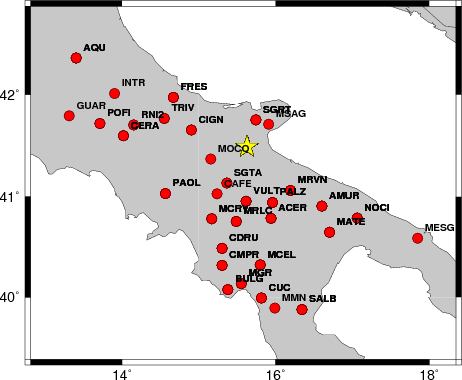
The focal mechanism was determined using broadband seismic waveforms. The location of the event and the
and stations used for the waveform inversion are shown in the next figure.
|
|
Location of broadband stations used for waveform inversion
|
The program wvfgrd96 was used with good traces observed at short distance to determine the focal mechanism, depth and seismic moment. This technique requires a high quality signal and well determined velocity model for the Green functions. To the extent that these are the quality data, this type of mechanism should be preferred over the radiation pattern technique which requires the separate step of defining the pressure and tension quadrants and the correct strike.
The observed and predicted traces are filtered using the following gsac commands:
hp c 0.02 n 3
lp c 0.10 n 3
The results of this grid search from 0.5 to 19 km depth are as follow:
           DEPTH  STK   DIP  RAKE   MW    FIT
WVFGRD96    1.0   295    50    85   3.65 0.2318
WVFGRD96    2.0   290    55    85   3.73 0.2284
WVFGRD96    3.0    75    80    40   3.67 0.2011
WVFGRD96    4.0   255    90   -40   3.68 0.2085
WVFGRD96    5.0   180    35    20   3.77 0.2223
WVFGRD96    6.0   175    35    10   3.78 0.2457
WVFGRD96    7.0   170    40     0   3.80 0.2726
WVFGRD96    8.0   170    45     5   3.79 0.2998
WVFGRD96    9.0   165    45   -10   3.81 0.3241
WVFGRD96   10.0   165    45   -10   3.83 0.3482
WVFGRD96   11.0   165    45   -10   3.86 0.3708
WVFGRD96   12.0   165    45   -10   3.87 0.3916
WVFGRD96   13.0   165    45   -10   3.89 0.4103
WVFGRD96   14.0   165    45   -10   3.91 0.4270
WVFGRD96   15.0   165    45   -10   3.96 0.4434
WVFGRD96   16.0   165    45    -5   3.97 0.4576
WVFGRD96   17.0   165    45    -5   3.99 0.4700
WVFGRD96   18.0   165    40    -5   4.00 0.4812
WVFGRD96   19.0   165    40    -5   4.02 0.4910
WVFGRD96   20.0   165    40    -5   4.03 0.4991
WVFGRD96   21.0   165    40    -5   4.05 0.5060
WVFGRD96   22.0   165    40    -5   4.06 0.5115
WVFGRD96   23.0   165    40    -5   4.07 0.5149
WVFGRD96   24.0   165    40    -5   4.08 0.5162
WVFGRD96   25.0   165    40    -5   4.09 0.5155
WVFGRD96   26.0   165    40    -5   4.10 0.5121
WVFGRD96   27.0   165    40    -5   4.11 0.5072
WVFGRD96   28.0   165    40    -5   4.11 0.5005
WVFGRD96   29.0   165    45    -5   4.12 0.4931
The best solution is
WVFGRD96 24.0 165 40 -5 4.08 0.5162
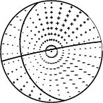
The mechanism correspond to the best fit is
|
|
Figure 1. Waveform inversion focal mechanism
|
The best fit as a function of depth is given in the following figure:
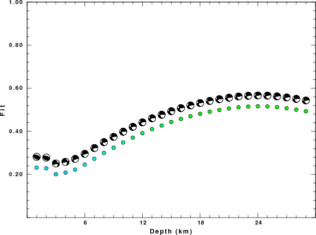
|
|
Figure 2. Depth sensitivity for waveform mechanism
|
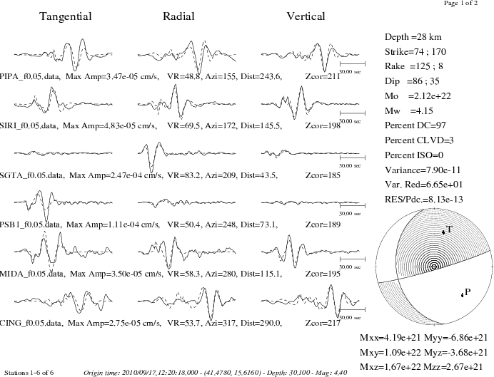
The comparison of the observed and predicted waveforms is given in the next figure. The red traces are the observed and the blue are the predicted.
Each observed-predicted component is plotted to the same scale and peak amplitudes are indicated by the numbers to the left of each trace. A pair of numbers is given in black at the right of each predicted traces. The upper number it the time shift required for maximum correlation between the observed and predicted traces. This time shift is required because the synthetics are not computed at exactly the same distance as the observed and because the velocity model used in the predictions may not be perfect.
A positive time shift indicates that the prediction is too fast and should be delayed to match the observed trace (shift to the right in this figure). A negative value indicates that the prediction is too slow. The lower number gives the percentage of variance reduction to characterize the individual goodness of fit (100% indicates a perfect fit).
The bandpass filter used in the processing and for the display was
hp c 0.02 n 3
lp c 0.10 n 3

|
|
Figure 3. Waveform comparison for selected depth
|
|
|
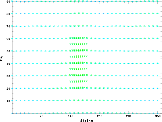
Focal mechanism sensitivity at the preferred depth. The red color indicates a very good fit to thewavefroms.
Each solution is plotted as a vector at a given value of strike and dip with the angle of the vector representing the rake angle, measured, with respect to the upward vertical (N) in the figure.
|
A check on the asusmed source location is possible by looking at the time shifts between the observed and predicted traces. The time shifts for waveform matching arise for several reasons:
- The origin time and epicentral distance are incorrect
- The velocity model used for hte inversion is incorrect
- The velocity model used to define the P-arrival time is not the
same as the velocity model used for the waveform inversion
(assuming that the initial trace alignment is based on the
P arrival time)
Assuming only a mislocation, the time shifts are fit to a functional form:
Time_shift = A + B cos Azimuth + C Sin Azimuth
The time shifst for this inversion lead to the next figure:
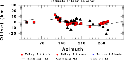
The derived shift in origin time and epicentral coordinates are given at the bottom of the figure.
Discussion
Velocity Model
The nnCIA used for the waveform synthetic seismograms and for the surface wave eigenfunctions and dispersion is as follows:
MODEL.01
C.It. A. Di Luzio et al Earth Plan Lettrs 280 (2009) 1-12 Fig 5. 7-8 MODEL/SURF3
ISOTROPIC
KGS
FLAT EARTH
1-D
CONSTANT VELOCITY
LINE08
LINE09
LINE10
LINE11
      H(KM)   VP(KM/S)   VS(KM/S) RHO(GM/CC)         QP         QS       ETAP       ETAS      FREFP      FREFS
     1.5000     3.7497     2.1436     2.2753  0.500E-02  0.100E-01   0.00       0.00       1.00       1.00
     3.0000     4.9399     2.8210     2.4858  0.500E-02  0.100E-01   0.00       0.00       1.00       1.00
     3.0000     6.0129     3.4336     2.7058  0.500E-02  0.100E-01   0.00       0.00       1.00       1.00
     7.0000     5.5516     3.1475     2.6093  0.167E-02  0.333E-02   0.00       0.00       1.00       1.00
    15.0000     5.8805     3.3583     2.6770  0.167E-02  0.333E-02   0.00       0.00       1.00       1.00
     6.0000     7.1059     4.0081     3.0002  0.167E-02  0.333E-02   0.00       0.00       1.00       1.00
     8.0000     7.1000     3.9864     3.0120  0.167E-02  0.333E-02   0.00       0.00       1.00       1.00
     0.0000     7.9000     4.4036     3.2760  0.167E-02  0.333E-02   0.00       0.00       1.00       1.00
Quality Control
Here we tabulate the reasons for not using certain digital data sets
The following stations did not have a valid response files:
DATE=Fri Sep 17 11:06:45 CDT 2010
Last Changed 2010/09/17