2010/09/01 13:11:32 42.840 12.671 2.4 2.9 Italy
USGS Felt map for this earthquake
 USGS/SLU Moment Tensor Solution
 ENS  2010/09/01 13:11:32:0  42.84   12.67   2.4 2.9 Italy

 Stations used:
   IV.AOI IV.ARVD IV.ASQU IV.ATPC IV.ATVO IV.CASP IV.CESI
   IV.CING IV.CRE IV.CSNT IV.FAGN IV.GUMA IV.LATE IV.MAON
   IV.MCIV IV.OFFI IV.PARC IV.POFI IV.SACS IV.SASS IV.SNTG
   IV.TERO MN.AQU

 Filtering commands used:
   hp c 0.02 n 3
   lp c 0.10 n 3

 Best Fitting Double Couple
  Mo = 9.44e+20 dyne-cm
  Mw = 3.25
  Z  = 6 km
  Plane   Strike  Dip  Rake
   NP1        5    80   -95
   NP2      212    11   -64
  Principal Axes:
   Axis    Value   Plunge  Azimuth
    T   9.44e+20     35      99
    N   0.00e+00      5       6
    P  -9.44e+20     55     269

 Moment Tensor: (dyne-cm)
    Component   Value
       Mxx     1.65e+19
       Mxy    -1.08e+20
       Mxz    -6.28e+19
       Myy     3.05e+20
       Myz     8.82e+20
       Mzz    -3.22e+20


                     #####----####-
                 ####---------#########
              ####-------------###########
             ##----------------############
           ###-----------------##############
          ##-------------------###############
         ##--------------------################
        ##---------------------#################
        ##---------------------#################
       ##----------------------##################
       ##---------   ----------##################
       ##--------- P ---------##########   ######
       ##---------   ---------########## T ######
        #---------------------##########   #####
        ##--------------------##################
         #--------------------#################
          #------------------#################
           #-----------------################
             ---------------###############
              #-------------##############
                 ----------############
                     ------########


 Global CMT Convention Moment Tensor:
      R          T          P
 -3.22e+20  -6.28e+19  -8.82e+20
 -6.28e+19   1.65e+19   1.08e+20
 -8.82e+20   1.08e+20   3.05e+20


Details of the solution is found at

http://www.eas.slu.edu/eqc/eqc_mt/MECH.IT/20100901131132/index.html
|
      STK = 5
      DIP = 80
     RAKE = -95
       MW = 3.25
       HS = 6.0
The waveform inversion is preferred.
The following compares this source inversion to others
 USGS/SLU Moment Tensor Solution
 ENS  2010/09/01 13:11:32:0  42.84   12.67   2.4 2.9 Italy

 Stations used:
   IV.AOI IV.ARVD IV.ASQU IV.ATPC IV.ATVO IV.CASP IV.CESI
   IV.CING IV.CRE IV.CSNT IV.FAGN IV.GUMA IV.LATE IV.MAON
   IV.MCIV IV.OFFI IV.PARC IV.POFI IV.SACS IV.SASS IV.SNTG
   IV.TERO MN.AQU

 Filtering commands used:
   hp c 0.02 n 3
   lp c 0.10 n 3

 Best Fitting Double Couple
  Mo = 9.44e+20 dyne-cm
  Mw = 3.25
  Z  = 6 km
  Plane   Strike  Dip  Rake
   NP1        5    80   -95
   NP2      212    11   -64
  Principal Axes:
   Axis    Value   Plunge  Azimuth
    T   9.44e+20     35      99
    N   0.00e+00      5       6
    P  -9.44e+20     55     269

 Moment Tensor: (dyne-cm)
    Component   Value
       Mxx     1.65e+19
       Mxy    -1.08e+20
       Mxz    -6.28e+19
       Myy     3.05e+20
       Myz     8.82e+20
       Mzz    -3.22e+20


                     #####----####-
                 ####---------#########
              ####-------------###########
             ##----------------############
           ###-----------------##############
          ##-------------------###############
         ##--------------------################
        ##---------------------#################
        ##---------------------#################
       ##----------------------##################
       ##---------   ----------##################
       ##--------- P ---------##########   ######
       ##---------   ---------########## T ######
        #---------------------##########   #####
        ##--------------------##################
         #--------------------#################
          #------------------#################
           #-----------------################
             ---------------###############
              #-------------##############
                 ----------############
                     ------########


 Global CMT Convention Moment Tensor:
      R          T          P
 -3.22e+20  -6.28e+19  -8.82e+20
 -6.28e+19   1.65e+19   1.08e+20
 -8.82e+20   1.08e+20   3.05e+20


Details of the solution is found at

http://www.eas.slu.edu/eqc/eqc_mt/MECH.IT/20100901131132/index.html
|
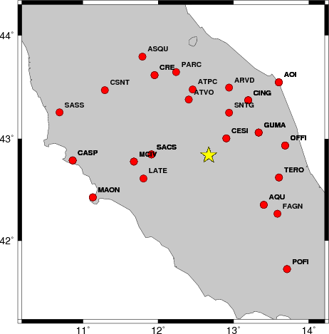
The focal mechanism was determined using broadband seismic waveforms. The location of the event and the and stations used for the waveform inversion are shown in the next figure.
|
|
|
|
The program wvfgrd96 was used with good traces observed at short distance to determine the focal mechanism, depth and seismic moment. This technique requires a high quality signal and well determined velocity model for the Green functions. To the extent that these are the quality data, this type of mechanism should be preferred over the radiation pattern technique which requires the separate step of defining the pressure and tension quadrants and the correct strike.
The observed and predicted traces are filtered using the following gsac commands:
hp c 0.02 n 3
lp c 0.10 n 3
The results of this grid search from 0.5 to 19 km depth are as follow:
           DEPTH  STK   DIP  RAKE   MW    FIT
WVFGRD96    1.0    10    35   -85   3.08 0.3493
WVFGRD96    2.0     5    85   -80   3.24 0.4067
WVFGRD96    3.0   185    90    80   3.19 0.5102
WVFGRD96    4.0   185    90    75   3.16 0.5536
WVFGRD96    5.0   185    90    80   3.26 0.5709
WVFGRD96    6.0     5    80   -95   3.25 0.5752
WVFGRD96    7.0   210    10   -65   3.24 0.5639
WVFGRD96    8.0   185    90    75   3.19 0.5427
WVFGRD96    9.0   180    90    70   3.20 0.5232
WVFGRD96   10.0     0    90   -70   3.21 0.5010
WVFGRD96   11.0   180    90    70   3.21 0.4768
WVFGRD96   12.0   185    85    70   3.22 0.4517
WVFGRD96   13.0   185    85    70   3.22 0.4275
WVFGRD96   14.0     5    90   -70   3.23 0.4040
WVFGRD96   15.0     0    90   -70   3.27 0.3808
WVFGRD96   16.0   185    85    75   3.27 0.3557
WVFGRD96   17.0   185    80    75   3.28 0.3311
WVFGRD96   18.0   175    65    70   3.29 0.3095
WVFGRD96   19.0   175    65    70   3.30 0.2927
WVFGRD96   20.0   175    60    70   3.30 0.2763
WVFGRD96   21.0   175    60    70   3.31 0.2610
WVFGRD96   22.0   175    60    70   3.31 0.2461
WVFGRD96   23.0   170    60    60   3.32 0.2330
WVFGRD96   24.0   170    60    60   3.33 0.2237
WVFGRD96   25.0   170    60    60   3.33 0.2165
WVFGRD96   26.0   175    55    65   3.33 0.2089
WVFGRD96   27.0    40    25   -55   3.34 0.2077
WVFGRD96   28.0    45    25   -50   3.35 0.2108
WVFGRD96   29.0    45    25   -50   3.36 0.2129
The best solution is
WVFGRD96 6.0 5 80 -95 3.25 0.5752
The mechanism correspond to the best fit is
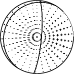
|
|
|
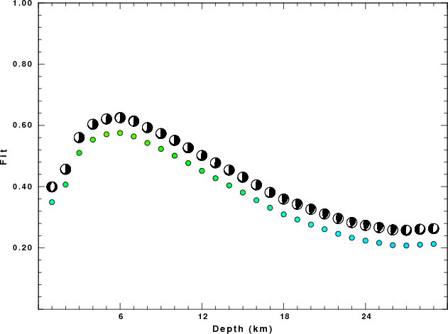
The best fit as a function of depth is given in the following figure:
|
|
|
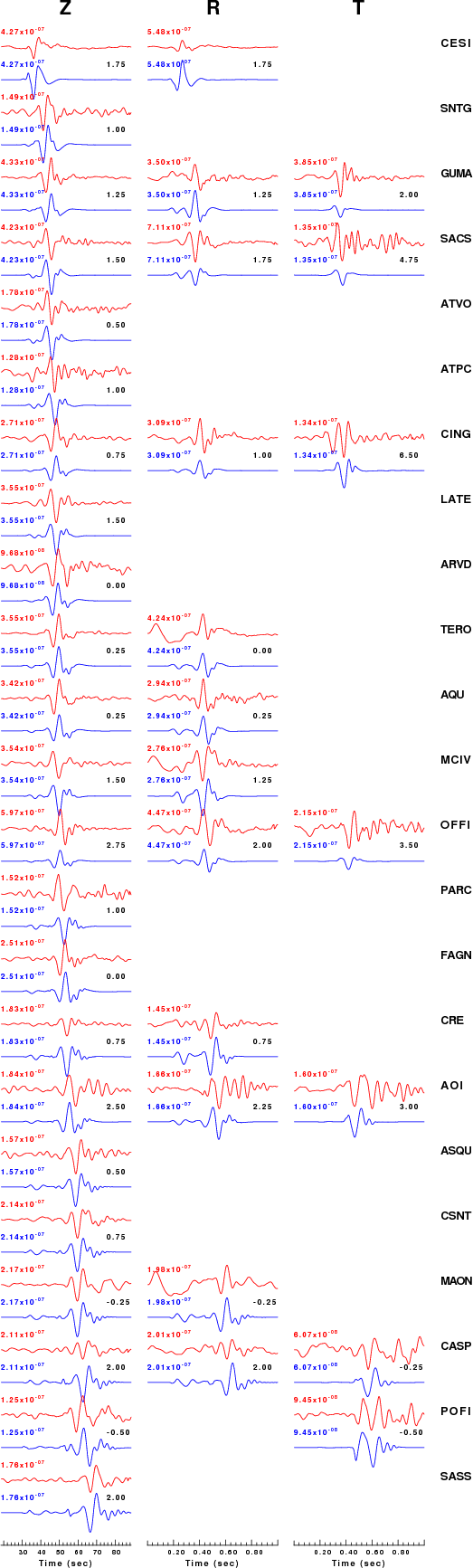
The comparison of the observed and predicted waveforms is given in the next figure. The red traces are the observed and the blue are the predicted. Each observed-predicted component is plotted to the same scale and peak amplitudes are indicated by the numbers to the left of each trace. The number in black at the rightr of each predicted traces it the time shift required for maximum correlation between the observed and predicted traces. This time shift is required because the synthetics are not computed at exactly the same distance as the observed and because the velocity model used in the predictions may not be perfect. A positive time shift indicates that the prediction is too fast and should be delayed to match the observed trace (shift to the right in this figure). A negative value indicates that the prediction is too slow. The bandpass filter used in the processing and for the display was
hp c 0.02 n 3
lp c 0.10 n 3
|
|
|
|
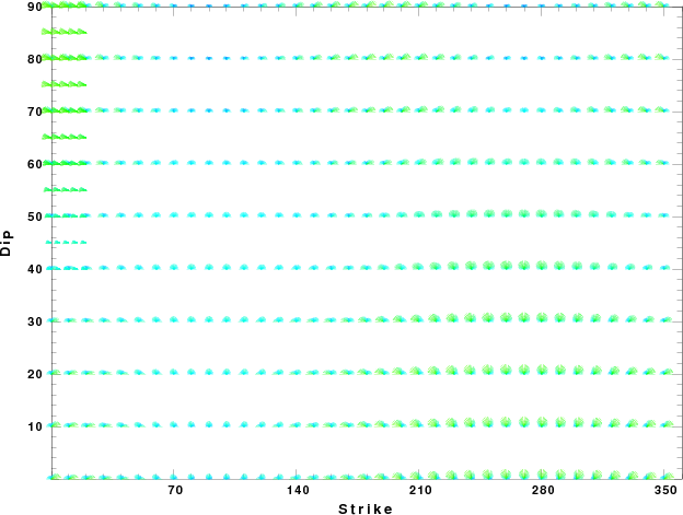
| Focal mechanism sensitivity at the preferred depth. The red color indicates a very good fit to thewavefroms. Each solution is plotted as a vector at a given value of strike and dip with the angle of the vector representing the rake angle, measured, with respect to the upward vertical (N) in the figure. |
The nnCIA used for the waveform synthetic seismograms and for the surface wave eigenfunctions and dispersion is as follows:
MODEL.01
C.It. A. Di Luzio et al Earth Plan Lettrs 280 (2009) 1-12 Fig 5. 7-8 MODEL/SURF3
ISOTROPIC
KGS
FLAT EARTH
1-D
CONSTANT VELOCITY
LINE08
LINE09
LINE10
LINE11
      H(KM)   VP(KM/S)   VS(KM/S) RHO(GM/CC)         QP         QS       ETAP       ETAS      FREFP      FREFS
     1.5000     3.7497     2.1436     2.2753  0.500E-02  0.100E-01   0.00       0.00       1.00       1.00
     3.0000     4.9399     2.8210     2.4858  0.500E-02  0.100E-01   0.00       0.00       1.00       1.00
     3.0000     6.0129     3.4336     2.7058  0.500E-02  0.100E-01   0.00       0.00       1.00       1.00
     7.0000     5.5516     3.1475     2.6093  0.167E-02  0.333E-02   0.00       0.00       1.00       1.00
    15.0000     5.8805     3.3583     2.6770  0.167E-02  0.333E-02   0.00       0.00       1.00       1.00
     6.0000     7.1059     4.0081     3.0002  0.167E-02  0.333E-02   0.00       0.00       1.00       1.00
     8.0000     7.1000     3.9864     3.0120  0.167E-02  0.333E-02   0.00       0.00       1.00       1.00
     0.0000     7.9000     4.4036     3.2760  0.167E-02  0.333E-02   0.00       0.00       1.00       1.00
Here we tabulate the reasons for not using certain digital data sets
The following stations did not have a valid response files:
DATE=Wed Sep 1 10:46:56 CDT 2010