2010/08/31 12:06:25 42.543 13.201 2.3 3.3 Italy
USGS Felt map for this earthquake
 USGS/SLU Moment Tensor Solution
 ENS  2010/08/31 12:06:25:0  42.54   13.20   2.3 3.3 Italy

 Stations used:
   IV.ARVD IV.CERT IV.CESI IV.CING IV.FAGN IV.FIAM IV.FSSB
   IV.GIUL IV.GUAR IV.GUMA IV.LATE IV.MGAB IV.MNS IV.MTCE
   IV.OFFI IV.PIEI IV.SACS IV.TOLF MN.AQU

 Filtering commands used:
   hp c 0.02 n 3
   lp c 0.10 n 3

 Best Fitting Double Couple
  Mo = 1.16e+21 dyne-cm
  Mw = 3.31
  Z  = 5 km
  Plane   Strike  Dip  Rake
   NP1      114    60   -93
   NP2      300    30   -85
  Principal Axes:
   Axis    Value   Plunge  Azimuth
    T   1.16e+21     15     206
    N   0.00e+00      2     116
    P  -1.16e+21     75      16

 Moment Tensor: (dyne-cm)
    Component   Value
       Mxx     7.95e+20
       Mxy     4.09e+20
       Mxz    -5.45e+20
       Myy     2.07e+20
       Myz    -2.13e+20
       Mzz    -1.00e+21


                     ##############
                 ######################
              ########----################
             ##------------------##########
           #------------------------#########
          -----------------------------#######
         --------------------------------######
        ##------------------   -----------######
        ###----------------- P -------------####
       #####----------------   --------------####
       #######-------------------------------####
       #########------------------------------###
       ###########----------------------------###
        #############-------------------------##
        ################-----------------------#
         ####################-----------------#
          ####################################
           ##################################
             #####   ######################
              #### T #####################
                 #   ##################
                     ##############


 Global CMT Convention Moment Tensor:
      R          T          P
 -1.00e+21  -5.45e+20   2.13e+20
 -5.45e+20   7.95e+20  -4.09e+20
  2.13e+20  -4.09e+20   2.07e+20


Details of the solution is found at

http://www.eas.slu.edu/eqc/eqc_mt/MECH.IT/20100831120625/index.html
|
      STK = 300
      DIP = 30
     RAKE = -85
       MW = 3.31
       HS = 5.0
The waveform inversion is preferred.
The following compares this source inversion to others
 USGS/SLU Moment Tensor Solution
 ENS  2010/08/31 12:06:25:0  42.54   13.20   2.3 3.3 Italy

 Stations used:
   IV.ARVD IV.CERT IV.CESI IV.CING IV.FAGN IV.FIAM IV.FSSB
   IV.GIUL IV.GUAR IV.GUMA IV.LATE IV.MGAB IV.MNS IV.MTCE
   IV.OFFI IV.PIEI IV.SACS IV.TOLF MN.AQU

 Filtering commands used:
   hp c 0.02 n 3
   lp c 0.10 n 3

 Best Fitting Double Couple
  Mo = 1.16e+21 dyne-cm
  Mw = 3.31
  Z  = 5 km
  Plane   Strike  Dip  Rake
   NP1      114    60   -93
   NP2      300    30   -85
  Principal Axes:
   Axis    Value   Plunge  Azimuth
    T   1.16e+21     15     206
    N   0.00e+00      2     116
    P  -1.16e+21     75      16

 Moment Tensor: (dyne-cm)
    Component   Value
       Mxx     7.95e+20
       Mxy     4.09e+20
       Mxz    -5.45e+20
       Myy     2.07e+20
       Myz    -2.13e+20
       Mzz    -1.00e+21


                     ##############
                 ######################
              ########----################
             ##------------------##########
           #------------------------#########
          -----------------------------#######
         --------------------------------######
        ##------------------   -----------######
        ###----------------- P -------------####
       #####----------------   --------------####
       #######-------------------------------####
       #########------------------------------###
       ###########----------------------------###
        #############-------------------------##
        ################-----------------------#
         ####################-----------------#
          ####################################
           ##################################
             #####   ######################
              #### T #####################
                 #   ##################
                     ##############


 Global CMT Convention Moment Tensor:
      R          T          P
 -1.00e+21  -5.45e+20   2.13e+20
 -5.45e+20   7.95e+20  -4.09e+20
  2.13e+20  -4.09e+20   2.07e+20


Details of the solution is found at

http://www.eas.slu.edu/eqc/eqc_mt/MECH.IT/20100831120625/index.html
|
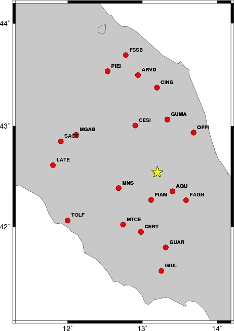
The focal mechanism was determined using broadband seismic waveforms. The location of the event and the and stations used for the waveform inversion are shown in the next figure.
|
|
|
|
The program wvfgrd96 was used with good traces observed at short distance to determine the focal mechanism, depth and seismic moment. This technique requires a high quality signal and well determined velocity model for the Green functions. To the extent that these are the quality data, this type of mechanism should be preferred over the radiation pattern technique which requires the separate step of defining the pressure and tension quadrants and the correct strike.
The observed and predicted traces are filtered using the following gsac commands:
hp c 0.02 n 3
lp c 0.10 n 3
The results of this grid search from 0.5 to 19 km depth are as follow:
           DEPTH  STK   DIP  RAKE   MW    FIT
WVFGRD96    1.0   330    25   -30   3.12 0.3245
WVFGRD96    2.0   325    20   -40   3.20 0.3910
WVFGRD96    3.0   310    25   -70   3.20 0.4511
WVFGRD96    4.0   300    30   -85   3.22 0.4867
WVFGRD96    5.0   300    30   -85   3.31 0.5057
WVFGRD96    6.0   305    35   -80   3.30 0.4811
WVFGRD96    7.0   105    60  -105   3.26 0.4297
WVFGRD96    8.0   315    35   -65   3.21 0.3686
WVFGRD96    9.0   340    70    20   3.23 0.3317
WVFGRD96   10.0   340    70    20   3.24 0.3160
WVFGRD96   11.0   340    70    20   3.25 0.2996
WVFGRD96   12.0   340    70    20   3.25 0.2831
WVFGRD96   13.0   345    70    25   3.26 0.2683
WVFGRD96   14.0   345    70    25   3.26 0.2545
WVFGRD96   15.0   345    65    25   3.28 0.2405
WVFGRD96   16.0   350    60    35   3.29 0.2313
WVFGRD96   17.0   350    60    35   3.30 0.2234
WVFGRD96   18.0   340    70    15   3.30 0.2175
WVFGRD96   19.0   345    60    25   3.31 0.2129
WVFGRD96   20.0   335    65   -25   3.28 0.2095
WVFGRD96   21.0   335    65   -25   3.29 0.2075
WVFGRD96   22.0   335    70   -20   3.31 0.2067
WVFGRD96   23.0   335    70   -20   3.32 0.2078
WVFGRD96   24.0   335    65   -25   3.32 0.2093
WVFGRD96   25.0   335    60   -25   3.33 0.2125
WVFGRD96   26.0   335    60   -25   3.35 0.2154
WVFGRD96   27.0   335    60   -25   3.36 0.2175
WVFGRD96   28.0   325    65   -40   3.37 0.2196
WVFGRD96   29.0   320    65   -40   3.39 0.2233
The best solution is
WVFGRD96 5.0 300 30 -85 3.31 0.5057
The mechanism correspond to the best fit is
|
|
|
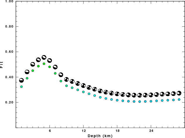
The best fit as a function of depth is given in the following figure:
|
|
|
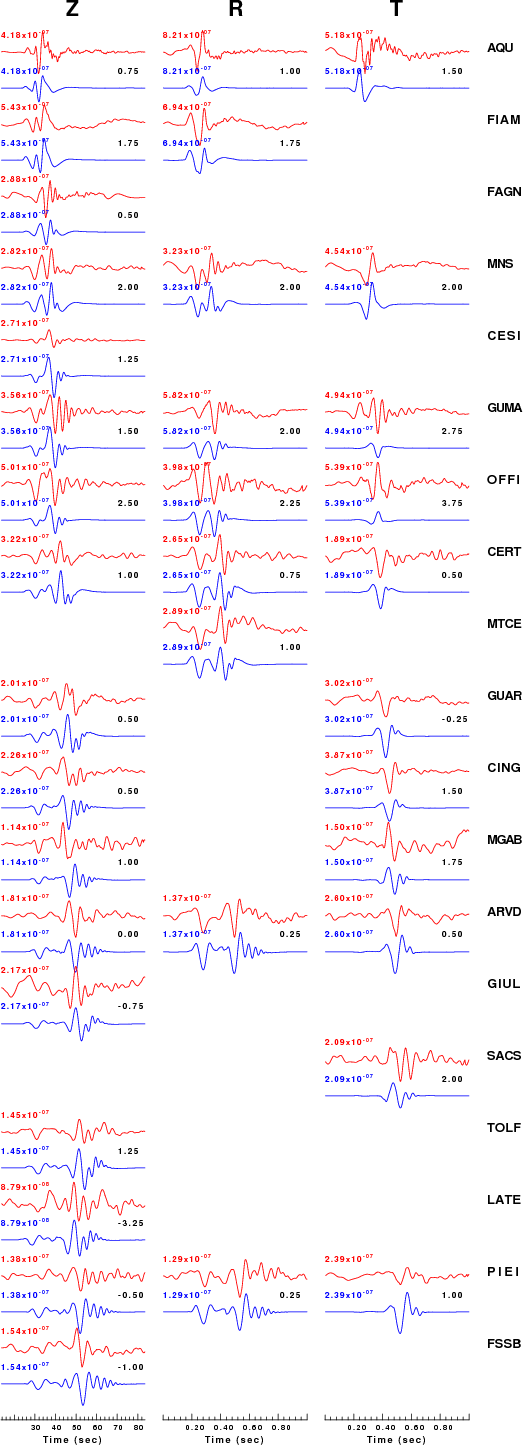
The comparison of the observed and predicted waveforms is given in the next figure. The red traces are the observed and the blue are the predicted. Each observed-predicted component is plotted to the same scale and peak amplitudes are indicated by the numbers to the left of each trace. The number in black at the rightr of each predicted traces it the time shift required for maximum correlation between the observed and predicted traces. This time shift is required because the synthetics are not computed at exactly the same distance as the observed and because the velocity model used in the predictions may not be perfect. A positive time shift indicates that the prediction is too fast and should be delayed to match the observed trace (shift to the right in this figure). A negative value indicates that the prediction is too slow. The bandpass filter used in the processing and for the display was
hp c 0.02 n 3
lp c 0.10 n 3
|
|
|
|
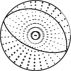
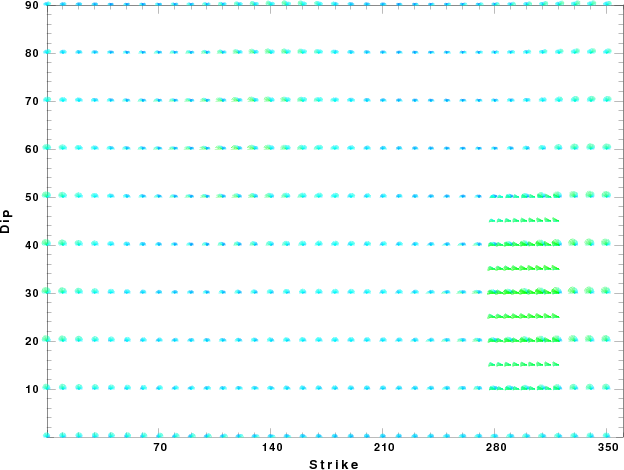
| Focal mechanism sensitivity at the preferred depth. The red color indicates a very good fit to thewavefroms. Each solution is plotted as a vector at a given value of strike and dip with the angle of the vector representing the rake angle, measured, with respect to the upward vertical (N) in the figure. |
The nnCIA used for the waveform synthetic seismograms and for the surface wave eigenfunctions and dispersion is as follows:
MODEL.01
C.It. A. Di Luzio et al Earth Plan Lettrs 280 (2009) 1-12 Fig 5. 7-8 MODEL/SURF3
ISOTROPIC
KGS
FLAT EARTH
1-D
CONSTANT VELOCITY
LINE08
LINE09
LINE10
LINE11
      H(KM)   VP(KM/S)   VS(KM/S) RHO(GM/CC)         QP         QS       ETAP       ETAS      FREFP      FREFS
     1.5000     3.7497     2.1436     2.2753  0.500E-02  0.100E-01   0.00       0.00       1.00       1.00
     3.0000     4.9399     2.8210     2.4858  0.500E-02  0.100E-01   0.00       0.00       1.00       1.00
     3.0000     6.0129     3.4336     2.7058  0.500E-02  0.100E-01   0.00       0.00       1.00       1.00
     7.0000     5.5516     3.1475     2.6093  0.167E-02  0.333E-02   0.00       0.00       1.00       1.00
    15.0000     5.8805     3.3583     2.6770  0.167E-02  0.333E-02   0.00       0.00       1.00       1.00
     6.0000     7.1059     4.0081     3.0002  0.167E-02  0.333E-02   0.00       0.00       1.00       1.00
     8.0000     7.1000     3.9864     3.0120  0.167E-02  0.333E-02   0.00       0.00       1.00       1.00
     0.0000     7.9000     4.4036     3.2760  0.167E-02  0.333E-02   0.00       0.00       1.00       1.00
Here we tabulate the reasons for not using certain digital data sets
The following stations did not have a valid response files:
DATE=Tue Aug 31 08:26:15 CDT 2010