Location
2010/07/13 03:36:18 40.581 15.452 10.4 3.4 Italy
Arrival Times (from USGS)
Arrival time list
Felt Map
USGS Felt map for this earthquake
USGS Felt reports page for
Focal Mechanism
 USGS/SLU Moment Tensor Solution
 ENS  2010/07/13 03:36:18:0  40.58   15.45  10.4 3.4 Italy

 Stations used:
   IV.BULG IV.CDRU IV.CMPR IV.MCEL IV.MCRV IV.MODR IV.MRVN
   IV.MSAG IV.PAOL IV.PSB1 IV.SGRT IV.SIRI MN.TIP

 Filtering commands used:
   hp c 0.02 n 3
   lp c 0.10 n 3

 Best Fitting Double Couple
  Mo = 2.75e+21 dyne-cm
  Mw = 3.56
  Z  = 7 km
  Plane   Strike  Dip  Rake
   NP1      340    70   -92
   NP2      165    20   -85
  Principal Axes:
   Axis    Value   Plunge  Azimuth
    T   2.75e+21     25      71
    N   0.00e+00      2     340
    P  -2.75e+21     65     247

 Moment Tensor: (dyne-cm)
    Component   Value
       Mxx     1.59e+20
       Mxy     5.12e+20
       Mxz     7.62e+20
       Myy     1.60e+21
       Myz     1.97e+21
       Mzz    -1.76e+21


                     ##############
                 ##----################
              ###--------#################
             ##-----------#################
           ###--------------#################
          ###----------------#################
         ###------------------#################
        ####-------------------##########   ####
        ###---------------------######### T ####
       ####---------------------#########   #####
       ####----------------------################
       ####---------   -----------###############
       ####--------- P -----------###############
        ####--------   ------------#############
        ####-----------------------#############
         ####----------------------############
          ####----------------------##########
           #####--------------------#########
             ####-------------------#######
              #####-----------------######
                 #####--------------###
                     ######--------


 Global CMT Convention Moment Tensor:
      R          T          P
 -1.76e+21   7.62e+20  -1.97e+21
  7.62e+20   1.59e+20  -5.12e+20
 -1.97e+21  -5.12e+20   1.60e+21


Details of the solution is found at

http://www.eas.slu.edu/eqc/eqc_mt/MECH.IT/20100713033618/index.html
|
Preferred Solution
The preferred solution from an analysis of the surface-wave spectral amplitude radiation pattern, waveform inversion and first motion observations is
      STK = 165
      DIP = 20
     RAKE = -85
       MW = 3.56
       HS = 7.0
The waveform inversion is preferred.
Moment Tensor Comparison
The following compares this source inversion to others
| SLU |
SLU |
 USGS/SLU Moment Tensor Solution
 ENS  2010/07/13 03:36:18:0  40.58   15.45  10.4 3.4 Italy

 Stations used:
   IV.BULG IV.CDRU IV.CMPR IV.MCEL IV.MCRV IV.MODR IV.MRVN
   IV.MSAG IV.PAOL IV.PSB1 IV.SGRT IV.SIRI MN.TIP

 Filtering commands used:
   hp c 0.02 n 3
   lp c 0.10 n 3

 Best Fitting Double Couple
  Mo = 2.75e+21 dyne-cm
  Mw = 3.56
  Z  = 7 km
  Plane   Strike  Dip  Rake
   NP1      340    70   -92
   NP2      165    20   -85
  Principal Axes:
   Axis    Value   Plunge  Azimuth
    T   2.75e+21     25      71
    N   0.00e+00      2     340
    P  -2.75e+21     65     247

 Moment Tensor: (dyne-cm)
    Component   Value
       Mxx     1.59e+20
       Mxy     5.12e+20
       Mxz     7.62e+20
       Myy     1.60e+21
       Myz     1.97e+21
       Mzz    -1.76e+21


                     ##############
                 ##----################
              ###--------#################
             ##-----------#################
           ###--------------#################
          ###----------------#################
         ###------------------#################
        ####-------------------##########   ####
        ###---------------------######### T ####
       ####---------------------#########   #####
       ####----------------------################
       ####---------   -----------###############
       ####--------- P -----------###############
        ####--------   ------------#############
        ####-----------------------#############
         ####----------------------############
          ####----------------------##########
           #####--------------------#########
             ####-------------------#######
              #####-----------------######
                 #####--------------###
                     ######--------


 Global CMT Convention Moment Tensor:
      R          T          P
 -1.76e+21   7.62e+20  -1.97e+21
  7.62e+20   1.59e+20  -5.12e+20
 -1.97e+21  -5.12e+20   1.60e+21


Details of the solution is found at

http://www.eas.slu.edu/eqc/eqc_mt/MECH.IT/20100713033618/index.html
|
SLU location using elocate is elocate.txt
|
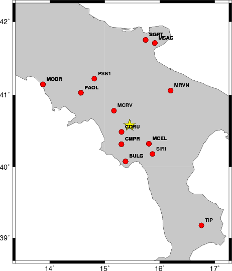
Waveform Inversion
The focal mechanism was determined using broadband seismic waveforms. The location of the event and the
and stations used for the waveform inversion are shown in the next figure.
|
|
Location of broadband stations used for waveform inversion
|
The program wvfgrd96 was used with good traces observed at short distance to determine the focal mechanism, depth and seismic moment. This technique requires a high quality signal and well determined velocity model for the Green functions. To the extent that these are the quality data, this type of mechanism should be preferred over the radiation pattern technique which requires the separate step of defining the pressure and tension quadrants and the correct strike.
The observed and predicted traces are filtered using the following gsac commands:
hp c 0.02 n 3
lp c 0.10 n 3
The results of this grid search from 0.5 to 19 km depth are as follow:
           DEPTH  STK   DIP  RAKE   MW    FIT
WVFGRD96    1.0   170    50   -15   3.32 0.3595
WVFGRD96    2.0   170    40   -15   3.41 0.4084
WVFGRD96    3.0   175    40    -5   3.42 0.4628
WVFGRD96    4.0   335    70   -85   3.44 0.5048
WVFGRD96    5.0   335    70   -90   3.54 0.5475
WVFGRD96    6.0   340    70   -90   3.55 0.5791
WVFGRD96    7.0   165    20   -85   3.56 0.5947
WVFGRD96    8.0   175    25   -75   3.53 0.5910
WVFGRD96    9.0   175    25   -75   3.54 0.5837
WVFGRD96   10.0   180    25   -70   3.55 0.5751
WVFGRD96   11.0   170    20   -80   3.55 0.5643
WVFGRD96   12.0   175    20   -75   3.56 0.5510
WVFGRD96   13.0   195    30   -45   3.57 0.5319
WVFGRD96   14.0   195    30   -45   3.58 0.5172
WVFGRD96   15.0   195    25   -50   3.63 0.5047
WVFGRD96   16.0   215    55    40   3.59 0.4933
WVFGRD96   17.0   215    55    40   3.60 0.4871
WVFGRD96   18.0   215    55    40   3.61 0.4779
WVFGRD96   19.0   220    50    40   3.62 0.4687
WVFGRD96   20.0   215    55    40   3.63 0.4591
WVFGRD96   21.0   220    50    40   3.63 0.4504
WVFGRD96   22.0   215    50    35   3.64 0.4443
WVFGRD96   23.0   220    50    45   3.65 0.4399
WVFGRD96   24.0   220    50    40   3.66 0.4365
WVFGRD96   25.0   220    50    40   3.67 0.4333
WVFGRD96   26.0   225    50    50   3.68 0.4295
WVFGRD96   27.0   225    50    45   3.69 0.4246
WVFGRD96   28.0   230    50    55   3.70 0.4192
WVFGRD96   29.0   230    50    50   3.71 0.4153
The best solution is
WVFGRD96 7.0 165 20 -85 3.56 0.5947
The mechanism correspond to the best fit is
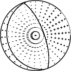
|
|
Figure 1. Waveform inversion focal mechanism
|
The best fit as a function of depth is given in the following figure:
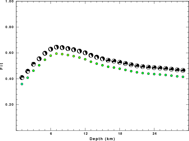
|
|
Figure 2. Depth sensitivity for waveform mechanism
|
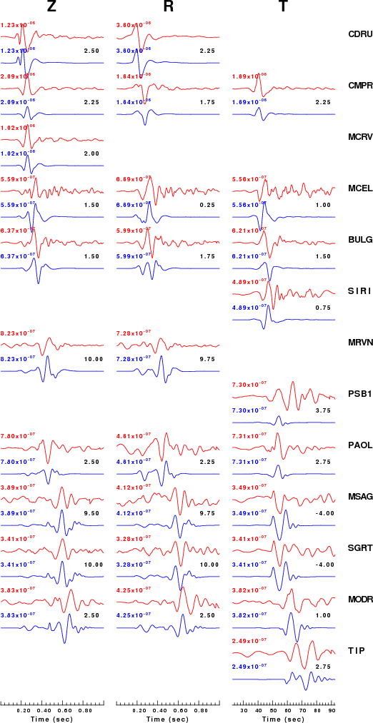
The comparison of the observed and predicted waveforms is given in the next figure. The red traces are the observed and the blue are the predicted.
Each observed-predicted component is plotted to the same scale and peak amplitudes are indicated by the numbers to the left of each trace. The number in black at the rightr of each predicted traces it the time shift required for maximum correlation between the observed and predicted traces. This time shift is required because the synthetics are not computed at exactly the same distance as the observed and because the velocity model used in the predictions may not be perfect.
A positive time shift indicates that the prediction is too fast and should be delayed to match the observed trace (shift to the right in this figure). A negative value indicates that the prediction is too slow.
The bandpass filter used in the processing and for the display was
hp c 0.02 n 3
lp c 0.10 n 3
|
|
Figure 3. Waveform comparison for selected depth
|
|
|
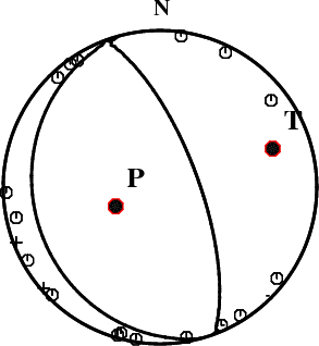
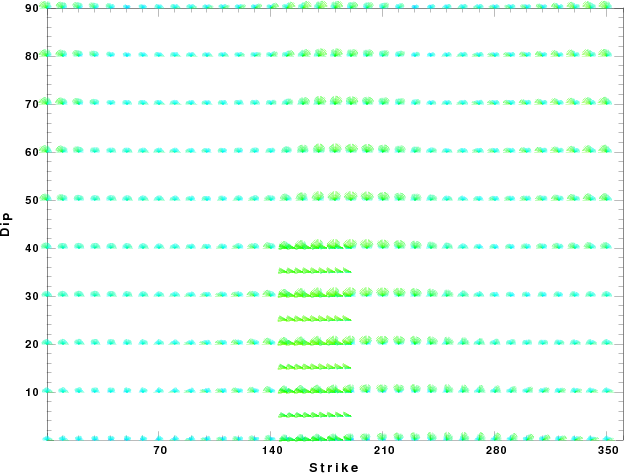
Focal mechanism sensitivity at the preferred depth. The red color indicates a very good fit to thewavefroms.
Each solution is plotted as a vector at a given value of strike and dip with the angle of the vector representing the rake angle, measured, with respect to the upward vertical (N) in the figure.
|
Discussion
Velocity Model
The nnCIA used for the waveform synthetic seismograms and for the surface wave eigenfunctions and dispersion is as follows:
MODEL.01
C.It. A. Di Luzio et al Earth Plan Lettrs 280 (2009) 1-12 Fig 5. 7-8 MODEL/SURF3
ISOTROPIC
KGS
FLAT EARTH
1-D
CONSTANT VELOCITY
LINE08
LINE09
LINE10
LINE11
      H(KM)   VP(KM/S)   VS(KM/S) RHO(GM/CC)         QP         QS       ETAP       ETAS      FREFP      FREFS
     1.5000     3.7497     2.1436     2.2753  0.500E-02  0.100E-01   0.00       0.00       1.00       1.00
     3.0000     4.9399     2.8210     2.4858  0.500E-02  0.100E-01   0.00       0.00       1.00       1.00
     3.0000     6.0129     3.4336     2.7058  0.500E-02  0.100E-01   0.00       0.00       1.00       1.00
     7.0000     5.5516     3.1475     2.6093  0.167E-02  0.333E-02   0.00       0.00       1.00       1.00
    15.0000     5.8805     3.3583     2.6770  0.167E-02  0.333E-02   0.00       0.00       1.00       1.00
     6.0000     7.1059     4.0081     3.0002  0.167E-02  0.333E-02   0.00       0.00       1.00       1.00
     8.0000     7.1000     3.9864     3.0120  0.167E-02  0.333E-02   0.00       0.00       1.00       1.00
     0.0000     7.9000     4.4036     3.2760  0.167E-02  0.333E-02   0.00       0.00       1.00       1.00
Quality Control
Here we tabulate the reasons for not using certain digital data sets
The following stations did not have a valid response files:
DATE=Tue Jul 13 09:26:46 CDT 2010
Last Changed 2010/07/13