Location
2010/04/15 01:47:36 43.477 12.425 9.1 3.7 Italy
Arrival Times (from USGS)
Arrival time list
Felt Map
USGS Felt map for this earthquake
USGS Felt reports page for
Focal Mechanism
 USGS/SLU Moment Tensor Solution
 ENS  2010/04/15 01:47:36:0  43.48   12.43   9.1 3.7 Italy

 Stations used:
   IV.ARVD IV.ASQU IV.CAFI IV.CASP IV.CESX IV.CING IV.CRE
   IV.CSNT IV.FDMO IV.FSSB IV.GUMA IV.LATE IV.MGAB IV.NRCA
   IV.OFFI IV.PARC IV.PESA IV.SACS MN.AQU

 Filtering commands used:
   hp c 0.02 n 3
   lp c 0.10 n 3

 Best Fitting Double Couple
  Mo = 5.13e+21 dyne-cm
  Mw = 3.74
  Z  = 5 km
  Plane   Strike  Dip  Rake
   NP1      315    60   -95
   NP2      145    30   -81
  Principal Axes:
   Axis    Value   Plunge  Azimuth
    T   5.13e+21     15      49
    N   0.00e+00      4     317
    P  -5.13e+21     74     212

 Moment Tensor: (dyne-cm)
    Component   Value
       Mxx     1.83e+21
       Mxy     2.21e+21
       Mxz     1.96e+21
       Myy     2.60e+21
       Myz     1.65e+21
       Mzz    -4.42e+21


                     ##############
                 ######################
              -###########################
             #------####################
           ##-----------################ T ##
          ###---------------############   ###
         ###------------------#################
        ####--------------------################
        ####----------------------##############
       #####------------------------#############
       #####-------------------------############
       ######------------   ----------###########
       ######------------ P ------------#########
        ######-----------   -------------#######
        #######--------------------------#######
         #######--------------------------#####
          #######-------------------------####
           ########------------------------##
             ########----------------------
              ##########------------------
                 #############--------#
                     ##############


 Global CMT Convention Moment Tensor:
      R          T          P
 -4.42e+21   1.96e+21  -1.65e+21
  1.96e+21   1.83e+21  -2.21e+21
 -1.65e+21  -2.21e+21   2.60e+21


Details of the solution is found at

http://www.eas.slu.edu/eqc/eqc_mt/MECH.IT/20100415014736/index.html
|
Preferred Solution
The preferred solution from an analysis of the surface-wave spectral amplitude radiation pattern, waveform inversion and first motion observations is
      STK = 315
      DIP = 60
     RAKE = -95
       MW = 3.74
       HS = 5.0
The waveform inversion is preferred.
Moment Tensor Comparison
The following compares this source inversion to others
| SLU |
TDMT |
RCMT |
 USGS/SLU Moment Tensor Solution
 ENS  2010/04/15 01:47:36:0  43.48   12.43   9.1 3.7 Italy

 Stations used:
   IV.ARVD IV.ASQU IV.CAFI IV.CASP IV.CESX IV.CING IV.CRE
   IV.CSNT IV.FDMO IV.FSSB IV.GUMA IV.LATE IV.MGAB IV.NRCA
   IV.OFFI IV.PARC IV.PESA IV.SACS MN.AQU

 Filtering commands used:
   hp c 0.02 n 3
   lp c 0.10 n 3

 Best Fitting Double Couple
  Mo = 5.13e+21 dyne-cm
  Mw = 3.74
  Z  = 5 km
  Plane   Strike  Dip  Rake
   NP1      315    60   -95
   NP2      145    30   -81
  Principal Axes:
   Axis    Value   Plunge  Azimuth
    T   5.13e+21     15      49
    N   0.00e+00      4     317
    P  -5.13e+21     74     212

 Moment Tensor: (dyne-cm)
    Component   Value
       Mxx     1.83e+21
       Mxy     2.21e+21
       Mxz     1.96e+21
       Myy     2.60e+21
       Myz     1.65e+21
       Mzz    -4.42e+21


                     ##############
                 ######################
              -###########################
             #------####################
           ##-----------################ T ##
          ###---------------############   ###
         ###------------------#################
        ####--------------------################
        ####----------------------##############
       #####------------------------#############
       #####-------------------------############
       ######------------   ----------###########
       ######------------ P ------------#########
        ######-----------   -------------#######
        #######--------------------------#######
         #######--------------------------#####
          #######-------------------------####
           ########------------------------##
             ########----------------------
              ##########------------------
                 #############--------#
                     ##############


 Global CMT Convention Moment Tensor:
      R          T          P
 -4.42e+21   1.96e+21  -1.65e+21
  1.96e+21   1.83e+21  -2.21e+21
 -1.65e+21  -2.21e+21   2.60e+21


Details of the solution is found at

http://www.eas.slu.edu/eqc/eqc_mt/MECH.IT/20100415014736/index.html
|
|
RCMT from ing Bologna


http://cnt.rm.ingv.it/data_id/2211882670/qrcmt.gif
|
Waveform Inversion
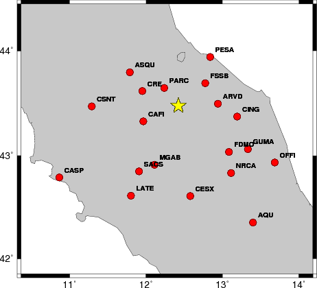
The focal mechanism was determined using broadband seismic waveforms. The location of the event and the
and stations used for the waveform inversion are shown in the next figure.
|
|
Location of broadband stations used for waveform inversion
|
The program wvfgrd96 was used with good traces observed at short distance to determine the focal mechanism, depth and seismic moment. This technique requires a high quality signal and well determined velocity model for the Green functions. To the extent that these are the quality data, this type of mechanism should be preferred over the radiation pattern technique which requires the separate step of defining the pressure and tension quadrants and the correct strike.
The observed and predicted traces are filtered using the following gsac commands:
hp c 0.02 n 3
lp c 0.10 n 3
The results of this grid search from 0.5 to 19 km depth are as follow:
           DEPTH  STK   DIP  RAKE   MW    FIT
WVFGRD96    1.0   160    30   -55   3.53 0.4183
WVFGRD96    2.0   330    70   -80   3.64 0.4789
WVFGRD96    3.0   320    60   -90   3.65 0.5321
WVFGRD96    4.0   315    60   -95   3.65 0.5427
WVFGRD96    5.0   315    60   -95   3.74 0.5756
WVFGRD96    6.0   145    30   -85   3.72 0.5088
WVFGRD96    7.0   170    35   -50   3.67 0.4448
WVFGRD96    8.0   185    70    20   3.64 0.4143
WVFGRD96    9.0   185    70    20   3.64 0.3988
WVFGRD96   10.0   190    70    20   3.64 0.3822
WVFGRD96   11.0   190    70    20   3.65 0.3688
WVFGRD96   12.0   190    70    20   3.65 0.3566
WVFGRD96   13.0   190    70    20   3.66 0.3464
WVFGRD96   14.0   190    65    20   3.67 0.3369
WVFGRD96   15.0   190    65    20   3.69 0.3227
WVFGRD96   16.0   190    65    20   3.70 0.3131
WVFGRD96   17.0     5    45   -20   3.71 0.3061
WVFGRD96   18.0     5    45   -20   3.72 0.3034
WVFGRD96   19.0     0    50   -20   3.74 0.3012
WVFGRD96   20.0     0    50   -20   3.75 0.3000
WVFGRD96   21.0     0    50   -25   3.76 0.2989
WVFGRD96   22.0     0    50   -25   3.77 0.2977
WVFGRD96   23.0     0    50   -25   3.78 0.2956
WVFGRD96   24.0    -5    50   -30   3.79 0.2929
WVFGRD96   25.0   125    55    70   3.79 0.2955
WVFGRD96   26.0   130    60    60   3.80 0.2989
WVFGRD96   27.0   130    60    60   3.81 0.3015
WVFGRD96   28.0   125    60    55   3.83 0.3013
WVFGRD96   29.0   125    60    55   3.84 0.3004
The best solution is
WVFGRD96 5.0 315 60 -95 3.74 0.5756
The mechanism correspond to the best fit is
|
|
Figure 1. Waveform inversion focal mechanism
|
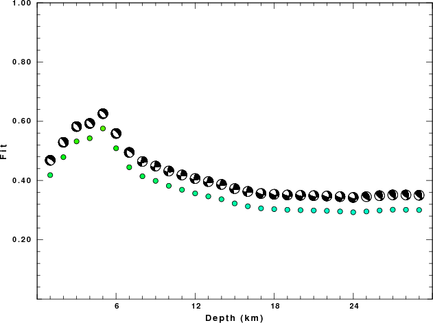
The best fit as a function of depth is given in the following figure:
|
|
Figure 2. Depth sensitivity for waveform mechanism
|
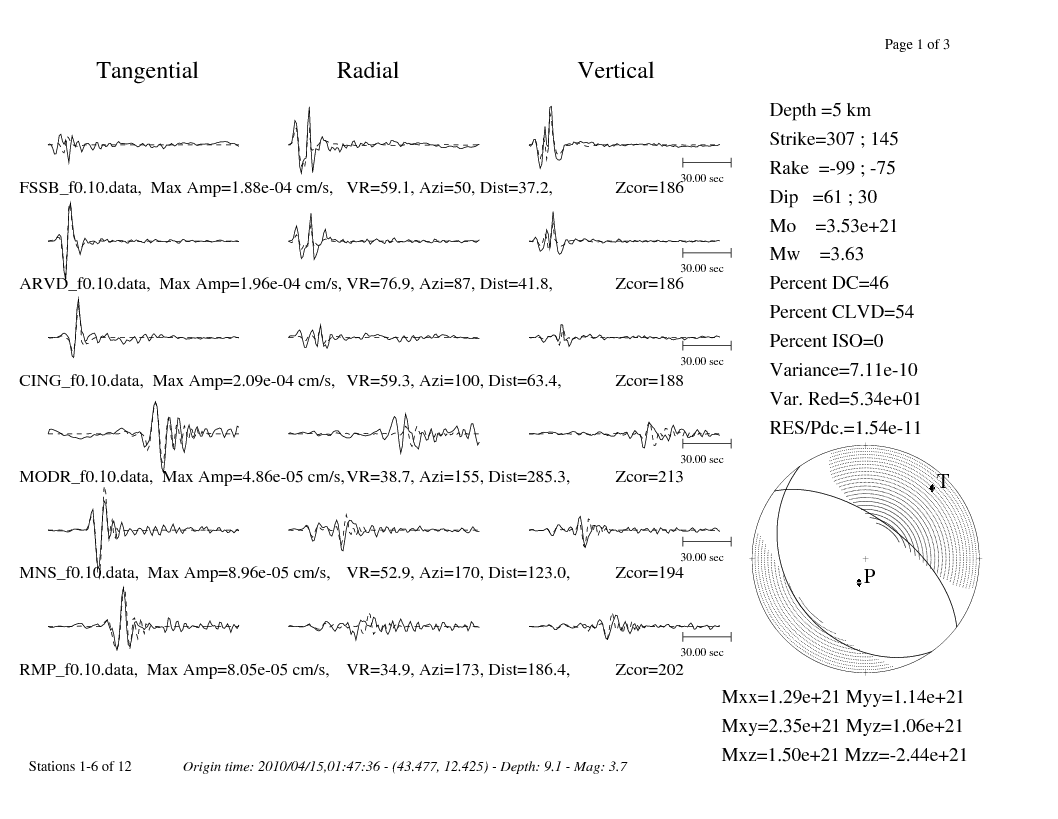
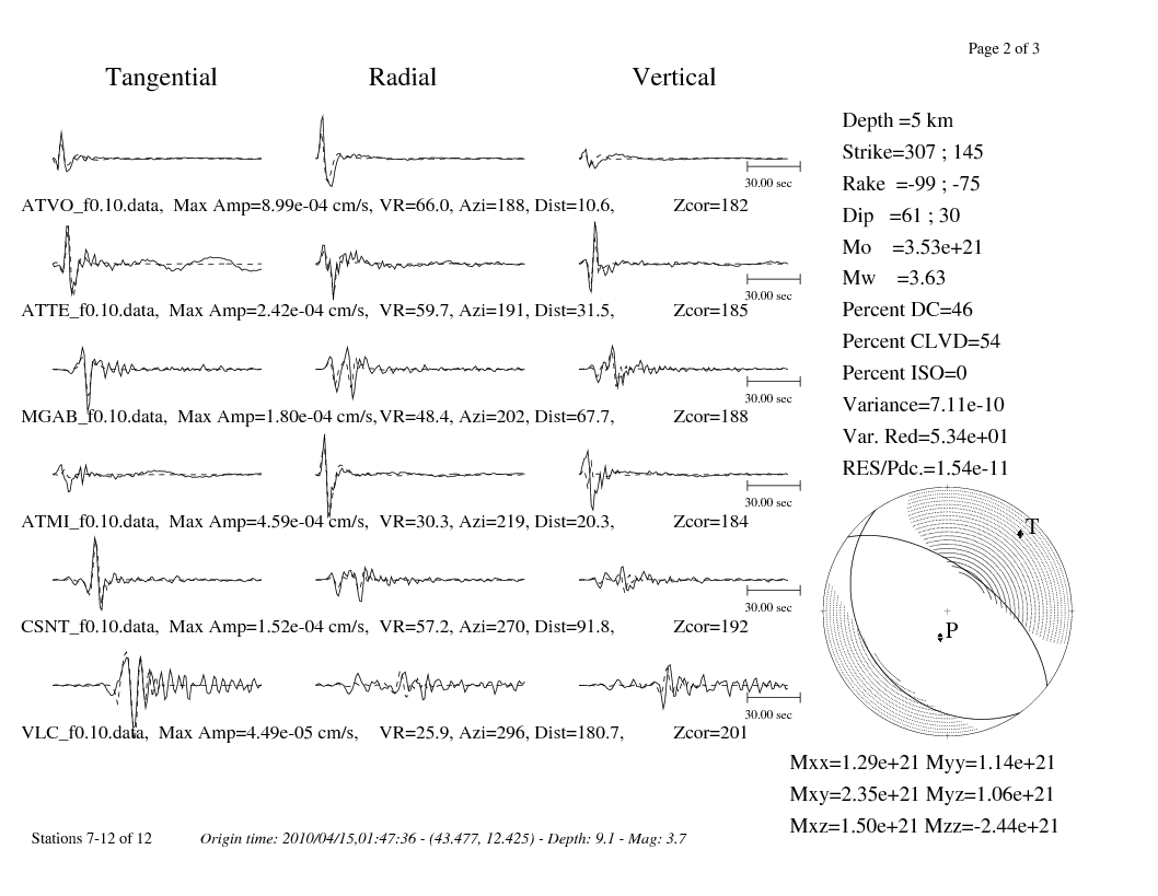
The comparison of the observed and predicted waveforms is given in the next figure. The red traces are the observed and the blue are the predicted.
Each observed-predicted component is plotted to the same scale and peak amplitudes are indicated by the numbers to the left of each trace. The number in black at the rightr of each predicted traces it the time shift required for maximum correlation between the observed and predicted traces. This time shift is required because the synthetics are not computed at exactly the same distance as the observed and because the velocity model used in the predictions may not be perfect.
A positive time shift indicates that the prediction is too fast and should be delayed to match the observed trace (shift to the right in this figure). A negative value indicates that the prediction is too slow.
The bandpass filter used in the processing and for the display was
hp c 0.02 n 3
lp c 0.10 n 3
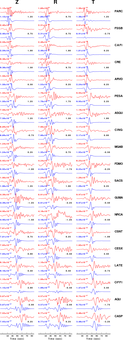
|
|
Figure 3. Waveform comparison for selected depth
|
|
|
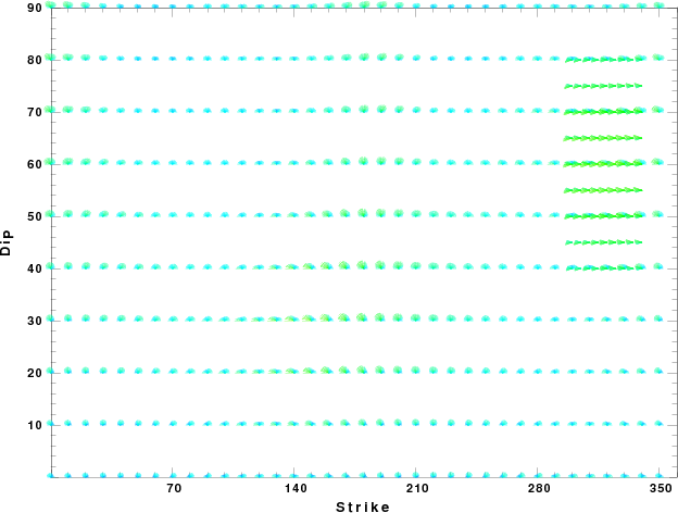
Focal mechanism sensitivity at the preferred depth. The red color indicates a very good fit to thewavefroms.
Each solution is plotted as a vector at a given value of strike and dip with the angle of the vector representing the rake angle, measured, with respect to the upward vertical (N) in the figure.
|
Discussion
Velocity Model
The nnCIA used for the waveform synthetic seismograms and for the surface wave eigenfunctions and dispersion is as follows:
MODEL.01
C.It. A. Di Luzio et al Earth Plan Lettrs 280 (2009) 1-12 Fig 5. 7-8 MODEL/SURF3
ISOTROPIC
KGS
FLAT EARTH
1-D
CONSTANT VELOCITY
LINE08
LINE09
LINE10
LINE11
      H(KM)   VP(KM/S)   VS(KM/S) RHO(GM/CC)         QP         QS       ETAP       ETAS      FREFP      FREFS
     1.5000     3.7497     2.1436     2.2753  0.500E-02  0.100E-01   0.00       0.00       1.00       1.00
     3.0000     4.9399     2.8210     2.4858  0.500E-02  0.100E-01   0.00       0.00       1.00       1.00
     3.0000     6.0129     3.4336     2.7058  0.500E-02  0.100E-01   0.00       0.00       1.00       1.00
     7.0000     5.5516     3.1475     2.6093  0.167E-02  0.333E-02   0.00       0.00       1.00       1.00
    15.0000     5.8805     3.3583     2.6770  0.167E-02  0.333E-02   0.00       0.00       1.00       1.00
     6.0000     7.1059     4.0081     3.0002  0.167E-02  0.333E-02   0.00       0.00       1.00       1.00
     8.0000     7.1000     3.9864     3.0120  0.167E-02  0.333E-02   0.00       0.00       1.00       1.00
     0.0000     7.9000     4.4036     3.2760  0.167E-02  0.333E-02   0.00       0.00       1.00       1.00
Quality Control
Here we tabulate the reasons for not using certain digital data sets
The following stations did not have a valid response files:
DATE=Mon May 17 08:32:36 CDT 2010
Last Changed 2010/04/15