2009/10/19 10:08:50 44.76 9.735 25.8 3.9 Italy
 STA  COMP DIS(K) AZM  AIN    ARR TIME             RES(SEC) WT QFM PHASE    WGT
 BOB    Z   28.47 269. 132. 20091019100856.047         0.02  0 iC P        0.95
 BOB    Z   28.47 269. 132. 20091019100901.261        -0.16  2 eX S        0.37
 PRMA   Z   40.05  91. 122. 20091019100857.746         0.14  2 e- P        0.38
 SC2M   Z   46.46 208. 118. 20091019100858.609         0.06  0 iD P        0.89
 MSSA   Z   55.86 204. 114. 20091019100859.957        -0.04  0 iD P        0.83
 VLC    Z   82.41 146.  55. 20091019100903.653        -0.24  0 iD P        0.40
 BDI    Z  101.04 141.  55. 20091019100906.516         0.00  0 iD P        0.49
 PCP    Z  103.40 256.  55. 20091019100907.216         0.37  2 e- P        0.13
 ZCCA   Z  104.11 116.  55. 20091019100909.205         2.26  2 eX P        0.02
 ROVR   Z  138.84  45.  55. 20091019100911.502        -0.33  0 iC P        0.20
 MABI   Z  152.71  21.  55. 20091019100913.313        -0.47  2 e- P        0.08
 RORO   Z  156.91 243.  55. 20091019100914.106        -0.27  2 e- P        0.10
 TUE    Z  192.11 349.  48. 20091019100919.073         0.22  0 iD P        0.18
 BRMO   Z  194.23  13.  48. 20091019100919.322         0.20  2 eX P        0.09
 BLB    Z  201.38 273.  48. 20091019100920.001        -0.03  2 eX P        0.12
 DOI    Z  205.36 263.  48. 20091019100921.562         1.03  2 e- P        0.03
 RETURN FOR NEXT SCREEN


 Error Ellipse  X=   0.7484 km  Y= 0.8221 km  Theta = 127.2335 deg

 RMS Error        :               0.067              sec
 Travel_Time_Table:          nnCIA
 Latitude         :             44.7741 +-    0.0071 N         0.7959 km
 Longitude        :              9.8073 +-    0.0099 E         0.7762 km
 Depth            :               27.77 +-      0.81 km
 Epoch Time       :      1255946928.866 +-      0.08 sec
 Event Time       :  20091019100848.866 +-      0.08 sec
 Event (OCAL)     :  2009 10 19 10 08 48 866
 HYPO71 Quality   :                  BB
 Gap              :                  76              deg
 USGS/SLU Moment Tensor Solution
 ENS  2009/10/19 10:08:50:0  44.76    9.73  25.8 3.9 Italy

 Stations used:
   IG.PCP IG.SC2M IV.BDI IV.BOB IV.MAGA IV.MSSA IV.PRMA
   IV.ROVR IV.ZCCA MN.VLC

 Filtering commands used:
   hp c 0.02 n 3
   lp c 0.10 n 3

 Best Fitting Double Couple
  Mo = 5.50e+21 dyne-cm
  Mw = 3.76
  Z  = 23 km
  Plane   Strike  Dip  Rake
   NP1      255    60   125
   NP2       20    45    45
  Principal Axes:
   Axis    Value   Plunge  Azimuth
    T   5.50e+21     59     216
    N   0.00e+00     30      55
    P  -5.50e+21      8     320

 Moment Tensor: (dyne-cm)
    Component   Value
       Mxx    -2.22e+21
       Mxy     3.35e+21
       Mxz    -2.58e+21
       Myy    -1.67e+21
       Myz    -9.40e+20
       Mzz     3.89e+21


                     --------------
                 --------------------##
                 ---------------------####
             - P ----------------------####
           ---   ----------------------######
          ------------------------------######
         ----------------------################
        ---------------#################------##
        -----------#####################--------
       ---------########################---------
       ------###########################---------
       ----############################----------
       ---#############################----------
        ##############   #############----------
        ############## T ############-----------
         #############   ###########-----------
          #########################-----------
           #######################-----------
             ###################-----------
              ################------------
                 ##########------------
                     #-------------


 Global CMT Convention Moment Tensor:
      R          T          P
  3.89e+21  -2.58e+21   9.40e+20
 -2.58e+21  -2.22e+21  -3.35e+21
  9.40e+20  -3.35e+21  -1.67e+21


Details of the solution is found at

http://www.eas.slu.edu/eqc/eqc_mt/MECH.IT/20091019100850/index.html
|
      STK = 20
      DIP = 45
     RAKE = 45
       MW = 3.76
       HS = 23.0
The waveform inversion is preferred.
The following compares this source inversion to others
 USGS/SLU Moment Tensor Solution
 ENS  2009/10/19 10:08:50:0  44.76    9.73  25.8 3.9 Italy

 Stations used:
   IG.PCP IG.SC2M IV.BDI IV.BOB IV.MAGA IV.MSSA IV.PRMA
   IV.ROVR IV.ZCCA MN.VLC

 Filtering commands used:
   hp c 0.02 n 3
   lp c 0.10 n 3

 Best Fitting Double Couple
  Mo = 5.50e+21 dyne-cm
  Mw = 3.76
  Z  = 23 km
  Plane   Strike  Dip  Rake
   NP1      255    60   125
   NP2       20    45    45
  Principal Axes:
   Axis    Value   Plunge  Azimuth
    T   5.50e+21     59     216
    N   0.00e+00     30      55
    P  -5.50e+21      8     320

 Moment Tensor: (dyne-cm)
    Component   Value
       Mxx    -2.22e+21
       Mxy     3.35e+21
       Mxz    -2.58e+21
       Myy    -1.67e+21
       Myz    -9.40e+20
       Mzz     3.89e+21


                     --------------
                 --------------------##
                 ---------------------####
             - P ----------------------####
           ---   ----------------------######
          ------------------------------######
         ----------------------################
        ---------------#################------##
        -----------#####################--------
       ---------########################---------
       ------###########################---------
       ----############################----------
       ---#############################----------
        ##############   #############----------
        ############## T ############-----------
         #############   ###########-----------
          #########################-----------
           #######################-----------
             ###################-----------
              ################------------
                 ##########------------
                     #-------------


 Global CMT Convention Moment Tensor:
      R          T          P
  3.89e+21  -2.58e+21   9.40e+20
 -2.58e+21  -2.22e+21  -3.35e+21
  9.40e+20  -3.35e+21  -1.67e+21


Details of the solution is found at

http://www.eas.slu.edu/eqc/eqc_mt/MECH.IT/20091019100850/index.html
|
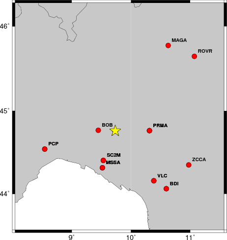
The focal mechanism was determined using broadband seismic waveforms. The location of the event and the and stations used for the waveform inversion are shown in the next figure.
|
|
|
|
The program wvfgrd96 was used with good traces observed at short distance to determine the focal mechanism, depth and seismic moment. This technique requires a high quality signal and well determined velocity model for the Green functions. To the extent that these are the quality data, this type of mechanism should be preferred over the radiation pattern technique which requires the separate step of defining the pressure and tension quadrants and the correct strike.
The observed and predicted traces are filtered using the following gsac commands:
hp c 0.02 n 3
lp c 0.10 n 3
The results of this grid search from 0.5 to 19 km depth are as follow:
           DEPTH  STK   DIP  RAKE   MW    FIT
WVFGRD96    1.0    40    45    85   3.36 0.2830
WVFGRD96    2.0   225    45    95   3.45 0.3054
WVFGRD96    3.0   180    90   -30   3.39 0.2687
WVFGRD96    4.0     0    90    25   3.43 0.2759
WVFGRD96    5.0   350    70   -40   3.50 0.2853
WVFGRD96    6.0   350    70   -45   3.52 0.2921
WVFGRD96    7.0   355    60   -40   3.54 0.3052
WVFGRD96    8.0    -5    60   -40   3.54 0.3222
WVFGRD96    9.0   355    60   -40   3.55 0.3368
WVFGRD96   10.0   355    60   -40   3.57 0.3493
WVFGRD96   11.0   355    65   -35   3.58 0.3595
WVFGRD96   12.0   355    65   -35   3.59 0.3684
WVFGRD96   13.0   350    65   -35   3.61 0.3767
WVFGRD96   14.0    15    60    35   3.62 0.3842
WVFGRD96   15.0    20    55    45   3.66 0.4052
WVFGRD96   16.0    20    55    45   3.67 0.4229
WVFGRD96   17.0    20    55    45   3.69 0.4389
WVFGRD96   18.0    20    50    45   3.70 0.4532
WVFGRD96   19.0    20    50    45   3.71 0.4655
WVFGRD96   20.0    20    50    45   3.73 0.4747
WVFGRD96   21.0    20    50    45   3.74 0.4824
WVFGRD96   22.0    20    50    45   3.75 0.4858
WVFGRD96   23.0    20    45    45   3.76 0.4862
WVFGRD96   24.0    20    45    45   3.77 0.4842
WVFGRD96   25.0    15    45    40   3.78 0.4834
WVFGRD96   26.0    20    40    45   3.78 0.4787
WVFGRD96   27.0    15    40    40   3.79 0.4741
WVFGRD96   28.0    15    40    40   3.80 0.4680
WVFGRD96   29.0    15    40    40   3.81 0.4601
The best solution is
WVFGRD96 23.0 20 45 45 3.76 0.4862
The mechanism correspond to the best fit is
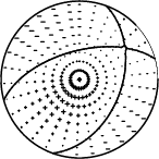
|
|
|
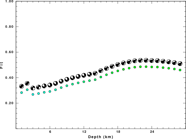
The best fit as a function of depth is given in the following figure:
|
|
|
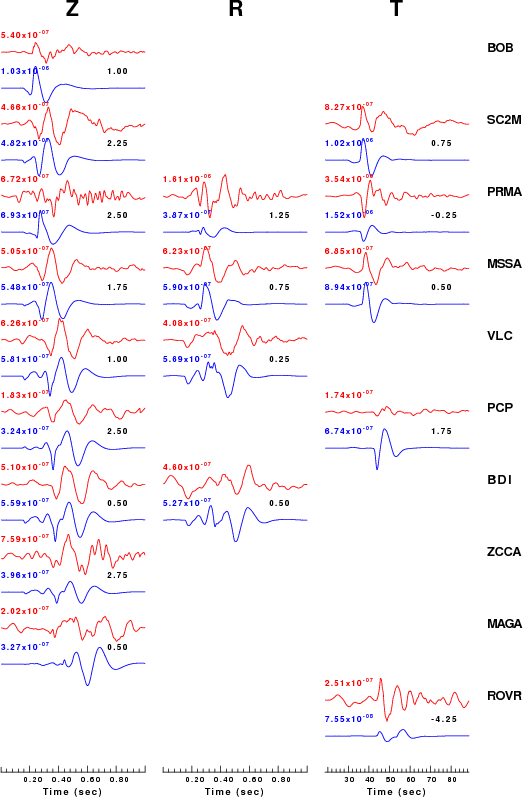
The comparison of the observed and predicted waveforms is given in the next figure. The red traces are the observed and the blue are the predicted. Each observed-predicted component is plotted to the same scale and peak amplitudes are indicated by the numbers to the left of each trace. The number in black at the rightr of each predicted traces it the time shift required for maximum correlation between the observed and predicted traces. This time shift is required because the synthetics are not computed at exactly the same distance as the observed and because the velocity model used in the predictions may not be perfect. A positive time shift indicates that the prediction is too fast and should be delayed to match the observed trace (shift to the right in this figure). A negative value indicates that the prediction is too slow. The bandpass filter used in the processing and for the display was
hp c 0.02 n 3
lp c 0.10 n 3
|
|
|
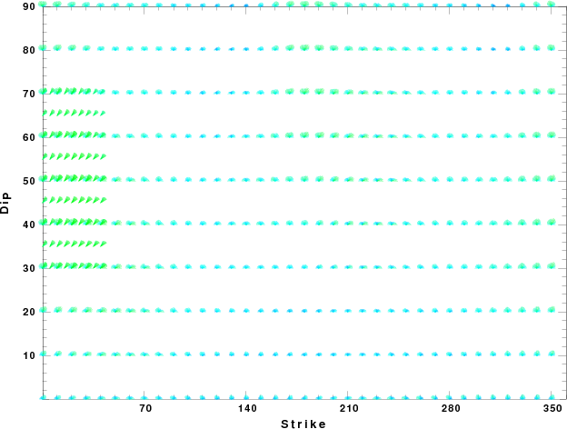
|
| Focal mechanism sensitivity at the preferred depth. The red color indicates a very good fit to thewavefroms. Each solution is plotted as a vector at a given value of strike and dip with the angle of the vector representing the rake angle, measured, with respect to the upward vertical (N) in the figure. |
The nnCIA used for the waveform synthetic seismograms and for the surface wave eigenfunctions and dispersion is as follows:
MODEL.01
C.It. A. Di Luzio et al Earth Plan Lettrs 280 (2009) 1-12 Fig 5. 7-8 MODEL/SURF3
ISOTROPIC
KGS
FLAT EARTH
1-D
CONSTANT VELOCITY
LINE08
LINE09
LINE10
LINE11
      H(KM)   VP(KM/S)   VS(KM/S) RHO(GM/CC)         QP         QS       ETAP       ETAS      FREFP      FREFS
     1.5000     3.7497     2.1436     2.2753  0.500E-02  0.100E-01   0.00       0.00       1.00       1.00
     3.0000     4.9399     2.8210     2.4858  0.500E-02  0.100E-01   0.00       0.00       1.00       1.00
     3.0000     6.0129     3.4336     2.7058  0.500E-02  0.100E-01   0.00       0.00       1.00       1.00
     7.0000     5.5516     3.1475     2.6093  0.167E-02  0.333E-02   0.00       0.00       1.00       1.00
    15.0000     5.8805     3.3583     2.6770  0.167E-02  0.333E-02   0.00       0.00       1.00       1.00
     6.0000     7.1059     4.0081     3.0002  0.167E-02  0.333E-02   0.00       0.00       1.00       1.00
     8.0000     7.1000     3.9864     3.0120  0.167E-02  0.333E-02   0.00       0.00       1.00       1.00
     0.0000     7.9000     4.4036     3.2760  0.167E-02  0.333E-02   0.00       0.00       1.00       1.00
Here we tabulate the reasons for not using certain digital data sets
The following stations did not have a valid response files:
DATE=Mon Oct 19 13:07:25 CDT 2009