2009/08/04 21:42:54 41.731 14.238 19.7 3.10 Italy
USGS Felt map for this earthquake
 USGS/SLU Moment Tensor Solution
 ENS  2009/08/04 21:42:54:0  41.73   14.24  19.7 3.1 Italy

 Stations used:
   IV.BSSO IV.CDRU IV.CERA IV.CERT IV.INTR IV.LPEL IV.MCRV
   IV.MELA IV.MNS IV.PSB1 IV.PTRJ IV.SGG IV.TERO MN.AQU

 Filtering commands used:
   hp c 0.02 n 3
   lp c 0.10 n 3

 Best Fitting Double Couple
  Mo = 1.05e+21 dyne-cm
  Mw = 3.28
  Z  = 15 km
  Plane   Strike  Dip  Rake
   NP1       30    80   -25
   NP2      125    65   -169
  Principal Axes:
   Axis    Value   Plunge  Azimuth
    T   1.05e+21     10      79
    N   0.00e+00     63     190
    P  -1.05e+21     25     345

 Moment Tensor: (dyne-cm)
    Component   Value
       Mxx    -7.72e+20
       Mxy     4.02e+20
       Mxz    -3.51e+20
       Myy     9.23e+20
       Myz     2.78e+20
       Mzz    -1.51e+20


                     --------------
                 -----   -------------#
              -------- P -------------####
             ---------   ------------######
           --------------------------########
          #-------------------------##########
         ###-----------------------############
        #####---------------------##############
        ######-------------------############
       #########----------------############# T #
       ##########--------------##############   #
       ############-----------###################
       ##############--------####################
        ################----####################
        ##################-#####################
         #################----#################
          ##############----------############
           ############----------------------
             #########---------------------
              ######----------------------
                 #---------------------
                     --------------


 Global CMT Convention Moment Tensor:
      R          T          P
 -1.51e+20  -3.51e+20  -2.78e+20
 -3.51e+20  -7.72e+20  -4.02e+20
 -2.78e+20  -4.02e+20   9.23e+20


Details of the solution is found at

http://www.eas.slu.edu/eqc/eqc_mt/MECH.IT/20090804214254/index.html
|
      STK = 30
      DIP = 80
     RAKE = -25
       MW = 3.28
       HS = 15.0
The waveform inversion is preferred.
The following compares this source inversion to others
 USGS/SLU Moment Tensor Solution
 ENS  2009/08/04 21:42:54:0  41.73   14.24  19.7 3.1 Italy

 Stations used:
   IV.BSSO IV.CDRU IV.CERA IV.CERT IV.INTR IV.LPEL IV.MCRV
   IV.MELA IV.MNS IV.PSB1 IV.PTRJ IV.SGG IV.TERO MN.AQU

 Filtering commands used:
   hp c 0.02 n 3
   lp c 0.10 n 3

 Best Fitting Double Couple
  Mo = 1.05e+21 dyne-cm
  Mw = 3.28
  Z  = 15 km
  Plane   Strike  Dip  Rake
   NP1       30    80   -25
   NP2      125    65   -169
  Principal Axes:
   Axis    Value   Plunge  Azimuth
    T   1.05e+21     10      79
    N   0.00e+00     63     190
    P  -1.05e+21     25     345

 Moment Tensor: (dyne-cm)
    Component   Value
       Mxx    -7.72e+20
       Mxy     4.02e+20
       Mxz    -3.51e+20
       Myy     9.23e+20
       Myz     2.78e+20
       Mzz    -1.51e+20


                     --------------
                 -----   -------------#
              -------- P -------------####
             ---------   ------------######
           --------------------------########
          #-------------------------##########
         ###-----------------------############
        #####---------------------##############
        ######-------------------############
       #########----------------############# T #
       ##########--------------##############   #
       ############-----------###################
       ##############--------####################
        ################----####################
        ##################-#####################
         #################----#################
          ##############----------############
           ############----------------------
             #########---------------------
              ######----------------------
                 #---------------------
                     --------------


 Global CMT Convention Moment Tensor:
      R          T          P
 -1.51e+20  -3.51e+20  -2.78e+20
 -3.51e+20  -7.72e+20  -4.02e+20
 -2.78e+20  -4.02e+20   9.23e+20


Details of the solution is found at

http://www.eas.slu.edu/eqc/eqc_mt/MECH.IT/20090804214254/index.html
|
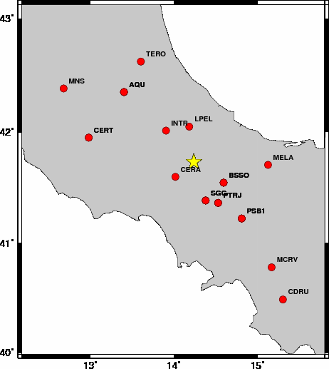
The focal mechanism was determined using broadband seismic waveforms. The location of the event and the and stations used for the waveform inversion are shown in the next figure.
|
|
|
|
The program wvfgrd96 was used with good traces observed at short distance to determine the focal mechanism, depth and seismic moment. This technique requires a high quality signal and well determined velocity model for the Green functions. To the extent that these are the quality data, this type of mechanism should be preferred over the radiation pattern technique which requires the separate step of defining the pressure and tension quadrants and the correct strike.
The observed and predicted traces are filtered using the following gsac commands:
hp c 0.02 n 3
lp c 0.10 n 3
The results of this grid search from 0.5 to 19 km depth are as follow:
           DEPTH  STK   DIP  RAKE   MW    FIT
WVFGRD96    0.5    75    45   -95   2.88 0.2524
WVFGRD96    1.0   260    45   -85   2.93 0.2514
WVFGRD96    2.0   260    65   -35   3.00 0.2591
WVFGRD96    3.0    30    75   -35   3.00 0.2645
WVFGRD96    4.0    30    70   -30   3.04 0.3122
WVFGRD96    5.0    25    70   -40   3.13 0.3509
WVFGRD96    6.0    30    75   -35   3.14 0.3869
WVFGRD96    7.0    30    75   -35   3.16 0.4205
WVFGRD96    8.0    30    80   -30   3.16 0.4506
WVFGRD96    9.0    30    80   -25   3.19 0.4761
WVFGRD96   10.0    30    80   -25   3.20 0.4963
WVFGRD96   11.0    35    90   -25   3.22 0.5123
WVFGRD96   12.0    35    90   -25   3.23 0.5238
WVFGRD96   13.0    35    90   -25   3.24 0.5304
WVFGRD96   14.0    35    90   -25   3.26 0.5341
WVFGRD96   15.0    30    80   -25   3.28 0.5352
WVFGRD96   16.0    35    85   -30   3.28 0.5339
WVFGRD96   17.0    35    85   -30   3.29 0.5304
WVFGRD96   18.0    35    85   -30   3.30 0.5253
WVFGRD96   19.0    30    75   -30   3.31 0.5195
WVFGRD96   20.0    30    75   -30   3.32 0.5124
WVFGRD96   21.0    30    75   -30   3.33 0.5043
WVFGRD96   22.0    30    75   -30   3.33 0.4950
WVFGRD96   23.0    30    75   -30   3.34 0.4850
WVFGRD96   24.0    30    75   -30   3.35 0.4742
WVFGRD96   25.0    30    70   -30   3.36 0.4643
WVFGRD96   26.0    30    70   -30   3.36 0.4542
WVFGRD96   27.0    25    65   -25   3.38 0.4464
WVFGRD96   28.0    25    65   -25   3.39 0.4400
WVFGRD96   29.0    25    60   -25   3.40 0.4362
The best solution is
WVFGRD96 15.0 30 80 -25 3.28 0.5352
The mechanism correspond to the best fit is
|
|
|
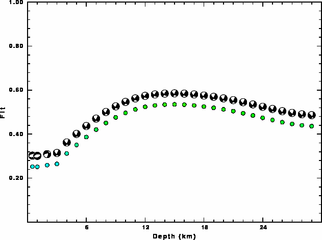
The best fit as a function of depth is given in the following figure:
|
|
|
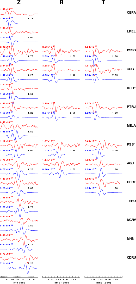
The comparison of the observed and predicted waveforms is given in the next figure. The red traces are the observed and the blue are the predicted. Each observed-predicted component is plotted to the same scale and peak amplitudes are indicated by the numbers to the left of each trace. The number in black at the rightr of each predicted traces it the time shift required for maximum correlation between the observed and predicted traces. This time shift is required because the synthetics are not computed at exactly the same distance as the observed and because the velocity model used in the predictions may not be perfect. A positive time shift indicates that the prediction is too fast and should be delayed to match the observed trace (shift to the right in this figure). A negative value indicates that the prediction is too slow. The bandpass filter used in the processing and for the display was
hp c 0.02 n 3
lp c 0.10 n 3
|
|
|
|
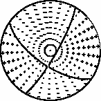
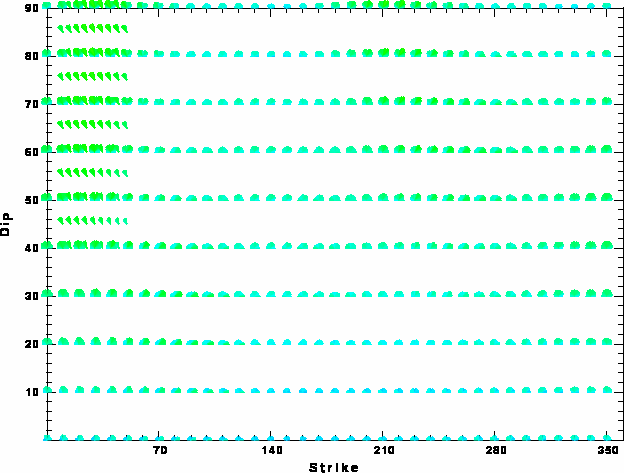
| Focal mechanism sensitivity at the preferred depth. The red color indicates a very good fit to thewavefroms. Each solution is plotted as a vector at a given value of strike and dip with the angle of the vector representing the rake angle, measured, with respect to the upward vertical (N) in the figure. |
The nnCIA used for the waveform synthetic seismograms and for the surface wave eigenfunctions and dispersion is as follows:
MODEL.01
C.It. A. Di Luzio et al Earth Plan Lettrs 280 (2009) 1-12 Fig 5. 7-8 MODEL/SURF3
ISOTROPIC
KGS
FLAT EARTH
1-D
CONSTANT VELOCITY
LINE08
LINE09
LINE10
LINE11
      H(KM)   VP(KM/S)   VS(KM/S) RHO(GM/CC)         QP         QS       ETAP       ETAS      FREFP      FREFS
     1.5000     3.7497     2.1436     2.2753  0.500E-02  0.100E-01   0.00       0.00       1.00       1.00
     3.0000     4.9399     2.8210     2.4858  0.500E-02  0.100E-01   0.00       0.00       1.00       1.00
     3.0000     6.0129     3.4336     2.7058  0.500E-02  0.100E-01   0.00       0.00       1.00       1.00
     7.0000     5.5516     3.1475     2.6093  0.167E-02  0.333E-02   0.00       0.00       1.00       1.00
    15.0000     5.8805     3.3583     2.6770  0.167E-02  0.333E-02   0.00       0.00       1.00       1.00
     6.0000     7.1059     4.0081     3.0002  0.167E-02  0.333E-02   0.00       0.00       1.00       1.00
     8.0000     7.1000     3.9864     3.0120  0.167E-02  0.333E-02   0.00       0.00       1.00       1.00
     0.0000     7.9000     4.4036     3.2760  0.167E-02  0.333E-02   0.00       0.00       1.00       1.00
Here we tabulate the reasons for not using certain digital data sets
The following stations did not have a valid response files:
DATE=Wed Aug 5 12:52:05 CDT 2009