2009/04/07 17:47:37 42.275 13.464 15.0 5.30 Italy
USGS Felt map for this earthquake
 USGS/SLU Moment Tensor Solution
 ENS  2009/04/07 17:47:37:0  42.28   13.46  15.0 5.3 Italy

 Stations used:
   IV.ARCI IV.BSSO IV.CAFR IV.CASP IV.CERT IV.CMPR IV.CRE
   IV.CSNT IV.GIUL IV.GUAR IV.LNSS IV.MAON IV.MCEL IV.MIDA
   IV.MNS IV.MODR IV.MSAG IV.MTCE IV.MTSN IV.MURB IV.NRCA
   IV.PARC IV.PESA IV.RMP IV.SGRT IV.SIRI IV.TOLF IV.TRIV

 Filtering commands used:
   hp c 0.02 n 3
   lp c 0.10 n 3

 Best Fitting Double Couple
  Mo = 2.24e+24 dyne-cm
  Mw = 5.50
  Z  = 18 km
  Plane   Strike  Dip  Rake
   NP1      340    75   -60
   NP2       94    33   -152
  Principal Axes:
   Axis    Value   Plunge  Azimuth
    T   2.24e+24     24      47
    N   0.00e+00     29     151
    P  -2.24e+24     51     284

 Moment Tensor: (dyne-cm)
    Component   Value
       Mxx     8.08e+23
       Mxy     1.14e+24
       Mxz     3.02e+23
       Myy     1.61e+23
       Myz     1.68e+24
       Mzz    -9.69e+23


                     ##############
                 ------################
              ----------##################
             -------------#################
           ----------------###########   ####
          ------------------########## T #####
         --------------------#########   ######
        ----------------------##################
        ---------   ----------##################
       ---------- P -----------##################
       ----------   ------------#################
       #------------------------#################
       ##------------------------###############-
        ##-----------------------##############-
        ####----------------------############--
         ####---------------------##########---
          ######-------------------#######----
           ########----------------###-------
             #############-----####--------
              #####################-------
                 ##################----
                     ##############


 Global CMT Convention Moment Tensor:
      R          T          P
 -9.69e+23   3.02e+23  -1.68e+24
  3.02e+23   8.08e+23  -1.14e+24
 -1.68e+24  -1.14e+24   1.61e+23


Details of the solution is found at

http://www.eas.slu.edu/eqc/eqc_mt/MECH.IT/20090407174737/index.html
|
      STK = 340
      DIP = 75
     RAKE = -60
       MW = 5.50
       HS = 18.0
The waveform inversion is preferred.
The following compares this source inversion to others
 USGS/SLU Moment Tensor Solution
 ENS  2009/04/07 17:47:37:0  42.28   13.46  15.0 5.3 Italy

 Stations used:
   IV.ARCI IV.BSSO IV.CAFR IV.CASP IV.CERT IV.CMPR IV.CRE
   IV.CSNT IV.GIUL IV.GUAR IV.LNSS IV.MAON IV.MCEL IV.MIDA
   IV.MNS IV.MODR IV.MSAG IV.MTCE IV.MTSN IV.MURB IV.NRCA
   IV.PARC IV.PESA IV.RMP IV.SGRT IV.SIRI IV.TOLF IV.TRIV

 Filtering commands used:
   hp c 0.02 n 3
   lp c 0.10 n 3

 Best Fitting Double Couple
  Mo = 2.24e+24 dyne-cm
  Mw = 5.50
  Z  = 18 km
  Plane   Strike  Dip  Rake
   NP1      340    75   -60
   NP2       94    33   -152
  Principal Axes:
   Axis    Value   Plunge  Azimuth
    T   2.24e+24     24      47
    N   0.00e+00     29     151
    P  -2.24e+24     51     284

 Moment Tensor: (dyne-cm)
    Component   Value
       Mxx     8.08e+23
       Mxy     1.14e+24
       Mxz     3.02e+23
       Myy     1.61e+23
       Myz     1.68e+24
       Mzz    -9.69e+23


                     ##############
                 ------################
              ----------##################
             -------------#################
           ----------------###########   ####
          ------------------########## T #####
         --------------------#########   ######
        ----------------------##################
        ---------   ----------##################
       ---------- P -----------##################
       ----------   ------------#################
       #------------------------#################
       ##------------------------###############-
        ##-----------------------##############-
        ####----------------------############--
         ####---------------------##########---
          ######-------------------#######----
           ########----------------###-------
             #############-----####--------
              #####################-------
                 ##################----
                     ##############


 Global CMT Convention Moment Tensor:
      R          T          P
 -9.69e+23   3.02e+23  -1.68e+24
  3.02e+23   8.08e+23  -1.14e+24
 -1.68e+24  -1.14e+24   1.61e+23


Details of the solution is found at

http://www.eas.slu.edu/eqc/eqc_mt/MECH.IT/20090407174737/index.html
|
April 7, 2009, CENTRAL ITALY, MW=5.5

Liz Starin

CENTROID-MOMENT-TENSOR  SOLUTION
GCMT EVENT:     C200904071747A
DATA: II IU CU G  GE
L.P.BODY WAVES: 65S, 111C, T= 40
MANTLE WAVES:   13S,  13C, T=125
SURFACE WAVES:  84S, 155C, T= 50
TIMESTAMP:      Q-20090407170307
CENTROID LOCATION:
ORIGIN TIME:      17:47:42.3 0.1
LAT:42.26N 0.01;LON: 13.46E 0.01
DEP: 20.0  0.5;TRIANG HDUR:  1.4
MOMENT TENSOR: SCALE 10**24 D-CM
RR=-1.630 0.038; TT= 0.767 0.030
PP= 0.865 0.031; RT=-0.763 0.066
RP=-1.120 0.071; TP=-1.590 0.026
PRINCIPAL AXES:
1.(T) VAL=  2.428;PLG= 4;AZM= 48
2.(N)       0.181;    36;    141
3.(P)      -2.607;    54;    312
BEST DBLE.COUPLE:M0= 2.52*10**24
NP1: STRIKE=106;DIP=51;SLIP=-138
NP2: STRIKE=347;DIP=59;SLIP= -47

            ---########
        ---------##########
      -------------#########
    ----------------######## T
   ------------------#######   #
  ---------   --------###########
  --------- P ---------##########
 #---------   ---------###########
 ##---------------------##########
 ####-------------------##########
 #####------------------##########
  #######---------------#########
  ##########------------#######--
   ################-------------
    ####################-------
      #################------
        ###############----
            ##########-
|
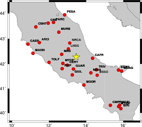
The focal mechanism was determined using broadband seismic waveforms. The location of the event and the and stations used for the waveform inversion are shown in the next figure.
|
|
|
|
The program wvfgrd96 was used with good traces observed at short distance to determine the focal mechanism, depth and seismic moment. This technique requires a high quality signal and well determined velocity model for the Green functions. To the extent that these are the quality data, this type of mechanism should be preferred over the radiation pattern technique which requires the separate step of defining the pressure and tension quadrants and the correct strike.
The observed and predicted traces are filtered using the following gsac commands:
hp c 0.02 n 3
lp c 0.10 n 3
The results of this grid search from 0.5 to 19 km depth are as follow:
           DEPTH  STK   DIP  RAKE   MW    FIT
WVFGRD96    0.5   330    45   -90   4.95 0.2175
WVFGRD96    1.0   150    45   -90   4.96 0.1730
WVFGRD96    2.0   330    45   -90   5.13 0.2486
WVFGRD96    3.0   170    70   -50   5.09 0.1827
WVFGRD96    4.0   175    90    60   5.14 0.2170
WVFGRD96    5.0   170    90    60   5.17 0.2712
WVFGRD96    6.0   170    90    60   5.20 0.3210
WVFGRD96    7.0   350    90   -55   5.22 0.3644
WVFGRD96    8.0   170    90    60   5.30 0.3988
WVFGRD96    9.0   345    80   -60   5.33 0.4441
WVFGRD96   10.0   340    75   -60   5.36 0.4836
WVFGRD96   11.0   340    75   -60   5.38 0.5191
WVFGRD96   12.0   340    75   -60   5.40 0.5488
WVFGRD96   13.0   340    75   -60   5.42 0.5732
WVFGRD96   14.0   340    75   -60   5.44 0.5925
WVFGRD96   15.0   340    75   -60   5.46 0.6068
WVFGRD96   16.0   340    75   -60   5.47 0.6164
WVFGRD96   17.0   340    75   -60   5.49 0.6219
WVFGRD96   18.0   340    75   -60   5.50 0.6232
WVFGRD96   19.0   340    75   -60   5.52 0.6212
WVFGRD96   20.0   340    75   -60   5.53 0.6164
WVFGRD96   21.0   340    75   -60   5.54 0.6095
WVFGRD96   22.0   340    75   -60   5.55 0.5995
WVFGRD96   23.0   340    75   -60   5.56 0.5875
WVFGRD96   24.0   340    75   -60   5.57 0.5737
WVFGRD96   25.0   340    75   -65   5.57 0.5589
WVFGRD96   26.0   340    75   -65   5.58 0.5432
WVFGRD96   27.0   340    75   -65   5.59 0.5265
WVFGRD96   28.0   340    75   -65   5.59 0.5096
WVFGRD96   29.0   340    75   -65   5.60 0.4923
The best solution is
WVFGRD96 18.0 340 75 -60 5.50 0.6232
The mechanism correspond to the best fit is
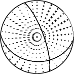
|
|
|
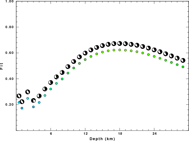
The best fit as a function of depth is given in the following figure:
|
|
|
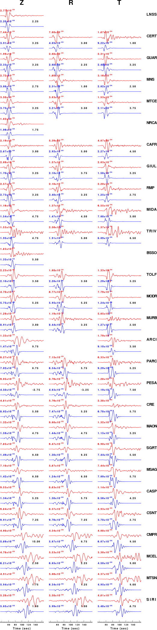
The comparison of the observed and predicted waveforms is given in the next figure. The red traces are the observed and the blue are the predicted. Each observed-predicted component is plotted to the same scale and peak amplitudes are indicated by the numbers to the left of each trace. The number in black at the rightr of each predicted traces it the time shift required for maximum correlation between the observed and predicted traces. This time shift is required because the synthetics are not computed at exactly the same distance as the observed and because the velocity model used in the predictions may not be perfect. A positive time shift indicates that the prediction is too fast and should be delayed to match the observed trace (shift to the right in this figure). A negative value indicates that the prediction is too slow. The bandpass filter used in the processing and for the display was
hp c 0.02 n 3
lp c 0.10 n 3
|
|
|
|
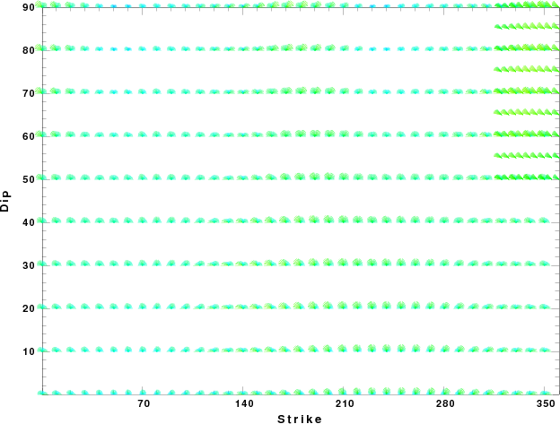
| Focal mechanism sensitivity at the preferred depth. The red color indicates a very good fit to thewavefroms. Each solution is plotted as a vector at a given value of strike and dip with the angle of the vector representing the rake angle, measured, with respect to the upward vertical (N) in the figure. |
The WUS used for the waveform synthetic seismograms and for the surface wave eigenfunctions and dispersion is as follows:
MODEL.01
Model after     8 iterations
ISOTROPIC
KGS
FLAT EARTH
1-D
CONSTANT VELOCITY
LINE08
LINE09
LINE10
LINE11
      H(KM)   VP(KM/S)   VS(KM/S) RHO(GM/CC)         QP         QS       ETAP       ETAS      FREFP      FREFS
     1.9000     3.4065     2.0089     2.2150  0.302E-02  0.679E-02   0.00       0.00       1.00       1.00
     6.1000     5.5445     3.2953     2.6089  0.349E-02  0.784E-02   0.00       0.00       1.00       1.00
    13.0000     6.2708     3.7396     2.7812  0.212E-02  0.476E-02   0.00       0.00       1.00       1.00
    19.0000     6.4075     3.7680     2.8223  0.111E-02  0.249E-02   0.00       0.00       1.00       1.00
     0.0000     7.9000     4.6200     3.2760  0.164E-10  0.370E-10   0.00       0.00       1.00       1.00
Here we tabulate the reasons for not using certain digital data sets
The following stations did not have a valid response files:
DATE=Mon Aug 31 14:56:03 CDT 2009