2009/04/06 23:15:37 42.4510 13.3640 8.0 4.80 Italy
USGS Felt map for this earthquake
 USGS/SLU Moment Tensor Solution
 ENS  2009/04/06 23:15:37:0  42.45   13.36   8.0 4.8 Italy

 Stations used:
   IG.MAIM IV.AMUR IV.AOI IV.ARVD IV.ASQU IV.BDI IV.BSSO
   IV.CAFI IV.CAFR IV.CASP IV.CERA IV.CERT IV.CESX IV.CING
   IV.CRMI IV.CSNT IV.FDMO IV.FRES IV.FSSB IV.GIUL IV.GUAR
   IV.MA9 IV.MAON IV.MGAB IV.MIDA IV.MIGL IV.MNS IV.MODR
   IV.MSAG IV.MTCE IV.MTRZ IV.MURB IV.OFFI IV.PESA IV.PIEI
   IV.POFI IV.PSB1 IV.PTRJ IV.RDP IV.RMP IV.ROM9 IV.SACS
   IV.SGRT IV.TERO IV.TOLF IV.TRIV IV.TRTR IV.VAGA IV.ZCCA
   MN.AQU

 Filtering commands used:
   hp c 0.02 n 3
   lp c 0.10 n 3

 Best Fitting Double Couple
  Mo = 3.24e+23 dyne-cm
  Mw = 4.94
  Z  = 9 km
  Plane   Strike  Dip  Rake
   NP1      327    51   -98
   NP2      160    40   -80
  Principal Axes:
   Axis    Value   Plunge  Azimuth
    T   3.24e+23      5      63
    N   0.00e+00      6     332
    P  -3.24e+23     82     193

 Moment Tensor: (dyne-cm)
    Component   Value
       Mxx     5.99e+22
       Mxy     1.29e+23
       Mxz     5.94e+22
       Myy     2.54e+23
       Myz     3.73e+22
       Mzz    -3.14e+23


                     ##############
                 --####################
              ####-------#################
             ####-----------###############
           #####--------------###############
          #####-----------------############
         ######-------------------########## T
        #######---------------------########   #
        #######----------------------###########
       ########-----------------------###########
       ########------------------------##########
       ########-----------   ----------##########
       #########---------- P -----------#########
        ########----------   -----------########
        #########------------------------#######
         #########-----------------------######
          #########----------------------#####
           ##########--------------------####
             ##########------------------##
              ###########---------------##
                 ###########-----------
                     #############-


 Global CMT Convention Moment Tensor:
      R          T          P
 -3.14e+23   5.94e+22  -3.73e+22
  5.94e+22   5.99e+22  -1.29e+23
 -3.73e+22  -1.29e+23   2.54e+23


Details of the solution is found at

http://www.eas.slu.edu/eqc/eqc_mt/MECH.IT/20090406231537/index.html
|
      STK = 160
      DIP = 40
     RAKE = -80
       MW = 4.94
       HS = 9.0
The waveform inversion is preferred.
The following compares this source inversion to others
 USGS/SLU Moment Tensor Solution
 ENS  2009/04/06 23:15:37:0  42.45   13.36   8.0 4.8 Italy

 Stations used:
   IG.MAIM IV.AMUR IV.AOI IV.ARVD IV.ASQU IV.BDI IV.BSSO
   IV.CAFI IV.CAFR IV.CASP IV.CERA IV.CERT IV.CESX IV.CING
   IV.CRMI IV.CSNT IV.FDMO IV.FRES IV.FSSB IV.GIUL IV.GUAR
   IV.MA9 IV.MAON IV.MGAB IV.MIDA IV.MIGL IV.MNS IV.MODR
   IV.MSAG IV.MTCE IV.MTRZ IV.MURB IV.OFFI IV.PESA IV.PIEI
   IV.POFI IV.PSB1 IV.PTRJ IV.RDP IV.RMP IV.ROM9 IV.SACS
   IV.SGRT IV.TERO IV.TOLF IV.TRIV IV.TRTR IV.VAGA IV.ZCCA
   MN.AQU

 Filtering commands used:
   hp c 0.02 n 3
   lp c 0.10 n 3

 Best Fitting Double Couple
  Mo = 3.24e+23 dyne-cm
  Mw = 4.94
  Z  = 9 km
  Plane   Strike  Dip  Rake
   NP1      327    51   -98
   NP2      160    40   -80
  Principal Axes:
   Axis    Value   Plunge  Azimuth
    T   3.24e+23      5      63
    N   0.00e+00      6     332
    P  -3.24e+23     82     193

 Moment Tensor: (dyne-cm)
    Component   Value
       Mxx     5.99e+22
       Mxy     1.29e+23
       Mxz     5.94e+22
       Myy     2.54e+23
       Myz     3.73e+22
       Mzz    -3.14e+23


                     ##############
                 --####################
              ####-------#################
             ####-----------###############
           #####--------------###############
          #####-----------------############
         ######-------------------########## T
        #######---------------------########   #
        #######----------------------###########
       ########-----------------------###########
       ########------------------------##########
       ########-----------   ----------##########
       #########---------- P -----------#########
        ########----------   -----------########
        #########------------------------#######
         #########-----------------------######
          #########----------------------#####
           ##########--------------------####
             ##########------------------##
              ###########---------------##
                 ###########-----------
                     #############-


 Global CMT Convention Moment Tensor:
      R          T          P
 -3.14e+23   5.94e+22  -3.73e+22
  5.94e+22   5.99e+22  -1.29e+23
 -3.73e+22  -1.29e+23   2.54e+23


Details of the solution is found at

http://www.eas.slu.edu/eqc/eqc_mt/MECH.IT/20090406231537/index.html
|
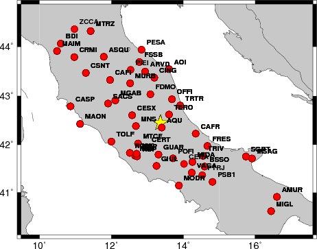
The focal mechanism was determined using broadband seismic waveforms. The location of the event and the and stations used for the waveform inversion are shown in the next figure.
|
|
|
|
The program wvfgrd96 was used with good traces observed at short distance to determine the focal mechanism, depth and seismic moment. This technique requires a high quality signal and well determined velocity model for the Green functions. To the extent that these are the quality data, this type of mechanism should be preferred over the radiation pattern technique which requires the separate step of defining the pressure and tension quadrants and the correct strike.
The observed and predicted traces are filtered using the following gsac commands:
hp c 0.02 n 3
lp c 0.10 n 3
The results of this grid search from 0.5 to 19 km depth are as follow:
           DEPTH  STK   DIP  RAKE   MW    FIT
WVFGRD96    0.5   150    45   -90   4.55 0.2587
WVFGRD96    1.0     0    55   -40   4.50 0.2022
WVFGRD96    2.0   345    45   -70   4.70 0.2644
WVFGRD96    3.0     5    30   -35   4.73 0.2788
WVFGRD96    4.0   205    25   -20   4.77 0.3297
WVFGRD96    5.0   200    25   -30   4.79 0.3703
WVFGRD96    6.0   200    30   -25   4.80 0.3974
WVFGRD96    7.0   200    35   -25   4.81 0.4124
WVFGRD96    8.0   190    30   -40   4.90 0.4258
WVFGRD96    9.0   160    40   -80   4.94 0.4330
WVFGRD96   10.0   165    45   -70   4.94 0.4323
WVFGRD96   11.0   165    45   -70   4.95 0.4259
WVFGRD96   12.0   165    50   -70   4.96 0.4161
WVFGRD96   13.0   165    50   -70   4.96 0.4040
WVFGRD96   14.0    10    60   -20   4.95 0.3992
WVFGRD96   15.0    10    60   -20   4.97 0.3941
WVFGRD96   16.0    10    60   -20   4.98 0.3869
WVFGRD96   17.0    10    60   -20   4.99 0.3786
WVFGRD96   18.0    10    60   -20   5.00 0.3697
WVFGRD96   19.0    10    60   -20   5.01 0.3602
WVFGRD96   20.0    10    60   -20   5.02 0.3498
WVFGRD96   21.0    10    60   -20   5.03 0.3414
WVFGRD96   22.0    15    55   -15   5.04 0.3321
WVFGRD96   23.0    15    55   -15   5.05 0.3239
WVFGRD96   24.0    15    55   -15   5.05 0.3153
WVFGRD96   25.0    15    55   -15   5.06 0.3065
WVFGRD96   26.0    20    50   -10   5.06 0.2986
WVFGRD96   27.0    20    50   -10   5.07 0.2917
WVFGRD96   28.0    20    45   -10   5.08 0.2854
WVFGRD96   29.0    25    45    -5   5.08 0.2788
The best solution is
WVFGRD96 9.0 160 40 -80 4.94 0.4330
The mechanism correspond to the best fit is
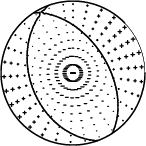
|
|
|
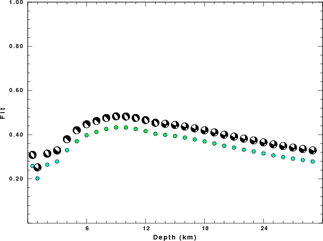
The best fit as a function of depth is given in the following figure:
|
|
|
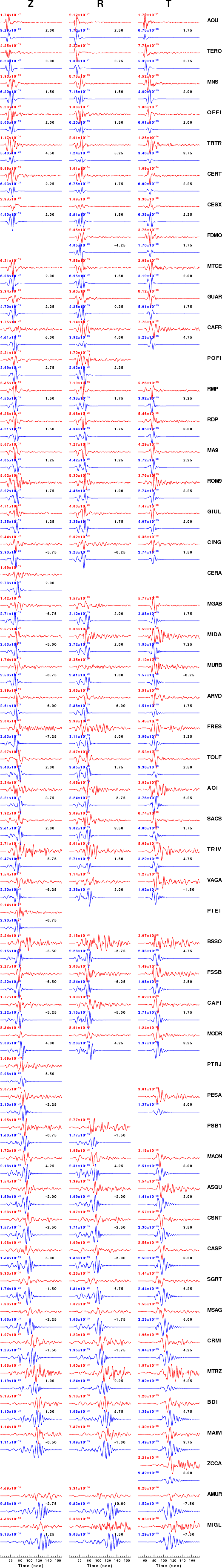
The comparison of the observed and predicted waveforms is given in the next figure. The red traces are the observed and the blue are the predicted. Each observed-predicted component is plotted to the same scale and peak amplitudes are indicated by the numbers to the left of each trace. The number in black at the rightr of each predicted traces it the time shift required for maximum correlation between the observed and predicted traces. This time shift is required because the synthetics are not computed at exactly the same distance as the observed and because the velocity model used in the predictions may not be perfect. A positive time shift indicates that the prediction is too fast and should be delayed to match the observed trace (shift to the right in this figure). A negative value indicates that the prediction is too slow. The bandpass filter used in the processing and for the display was
hp c 0.02 n 3
lp c 0.10 n 3
|
|
|
|
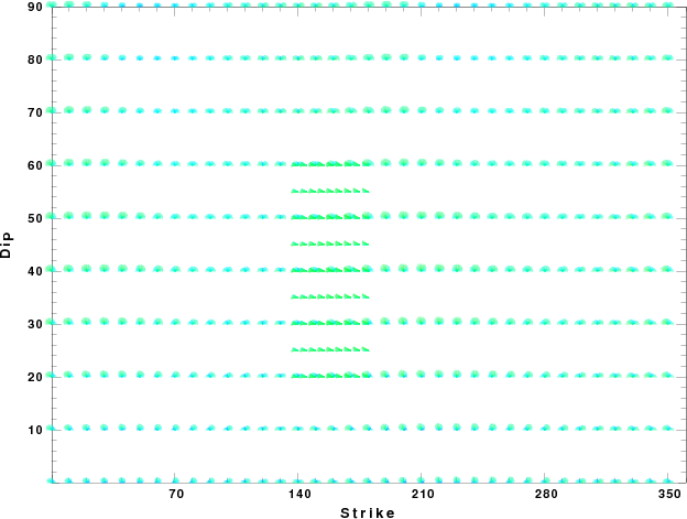
| Focal mechanism sensitivity at the preferred depth. The red color indicates a very good fit to thewavefroms. Each solution is plotted as a vector at a given value of strike and dip with the angle of the vector representing the rake angle, measured, with respect to the upward vertical (N) in the figure. |
The WUS used for the waveform synthetic seismograms and for the surface wave eigenfunctions and dispersion is as follows:
MODEL.01
Model after     8 iterations
ISOTROPIC
KGS
FLAT EARTH
1-D
CONSTANT VELOCITY
LINE08
LINE09
LINE10
LINE11
      H(KM)   VP(KM/S)   VS(KM/S) RHO(GM/CC)         QP         QS       ETAP       ETAS      FREFP      FREFS
     1.9000     3.4065     2.0089     2.2150  0.302E-02  0.679E-02   0.00       0.00       1.00       1.00
     6.1000     5.5445     3.2953     2.6089  0.349E-02  0.784E-02   0.00       0.00       1.00       1.00
    13.0000     6.2708     3.7396     2.7812  0.212E-02  0.476E-02   0.00       0.00       1.00       1.00
    19.0000     6.4075     3.7680     2.8223  0.111E-02  0.249E-02   0.00       0.00       1.00       1.00
     0.0000     7.9000     4.6200     3.2760  0.164E-10  0.370E-10   0.00       0.00       1.00       1.00
Here we tabulate the reasons for not using certain digital data sets
The following stations did not have a valid response files:
DATE=Mon Aug 31 14:48:39 CDT 2009