2009/04/06 03:56:45 42.336 13.387 10. 3.90 Italy
USGS Felt map for this earthquake
 USGS/SLU Moment Tensor Solution
 ENS  2009/04/06 03:56:45:0  42.34   13.39  10.0 3.9 Italy

 Stations used:
   IV.AOI IV.ARCI IV.ASQU IV.BSSO IV.CAFE IV.CAFI IV.CAFR
   IV.CERA IV.CERT IV.CESI IV.CING IV.FDMO IV.FSSB IV.GIUL
   IV.INTR IV.LATE IV.LPEL IV.MA9 IV.MAON IV.MGAB IV.MIDA
   IV.MODR IV.MRB1 IV.MTCE IV.MURB IV.NRCA IV.OFFI IV.PESA
   IV.PIEI IV.RMP IV.RNI2 IV.ROM9 IV.RSM IV.SGG IV.SGRT
   IV.TOLF IV.TRTR IV.VAGA IV.VVLD

 Filtering commands used:
   hp c 0.02 n 3
   lp c 0.10 n 3

 Best Fitting Double Couple
  Mo = 3.31e+22 dyne-cm
  Mw = 4.28
  Z  = 10 km
  Plane   Strike  Dip  Rake
   NP1      314    68   -118
   NP2      190    35   -40
  Principal Axes:
   Axis    Value   Plunge  Azimuth
    T   3.31e+22     19      65
    N   0.00e+00     26     326
    P  -3.31e+22     57     186

 Moment Tensor: (dyne-cm)
    Component   Value
       Mxx    -4.37e+21
       Mxy     1.03e+22
       Mxz     1.92e+22
       Myy     2.44e+22
       Myz     1.08e+22
       Mzz    -2.00e+22


                     -------#######
                 -------###############
              --------####################
             ###----#######################
           ########--########################
          #######-------######################
         ########----------###############   ##
        ########-------------############# T ###
        #######----------------###########   ###
       ########------------------################
       #######---------------------##############
       #######----------------------#############
       #######------------------------###########
        ######-------------------------#########
        #######-----------   -----------########
         ######----------- P ------------######
          ######----------   -------------####
           ######-------------------------###
             #####-------------------------
              #####-----------------------
                 ####------------------
                     ##------------


 Global CMT Convention Moment Tensor:
      R          T          P
 -2.00e+22   1.92e+22  -1.08e+22
  1.92e+22  -4.37e+21  -1.03e+22
 -1.08e+22  -1.03e+22   2.44e+22


Details of the solution is found at

http://www.eas.slu.edu/eqc/eqc_mt/MECH.IT/20090406035645/index.html
|
      STK = 190
      DIP = 35
     RAKE = -40
       MW = 4.28
       HS = 10.0
The waveform inversion is preferred.
The following compares this source inversion to others
 USGS/SLU Moment Tensor Solution
 ENS  2009/04/06 03:56:45:0  42.34   13.39  10.0 3.9 Italy

 Stations used:
   IV.AOI IV.ARCI IV.ASQU IV.BSSO IV.CAFE IV.CAFI IV.CAFR
   IV.CERA IV.CERT IV.CESI IV.CING IV.FDMO IV.FSSB IV.GIUL
   IV.INTR IV.LATE IV.LPEL IV.MA9 IV.MAON IV.MGAB IV.MIDA
   IV.MODR IV.MRB1 IV.MTCE IV.MURB IV.NRCA IV.OFFI IV.PESA
   IV.PIEI IV.RMP IV.RNI2 IV.ROM9 IV.RSM IV.SGG IV.SGRT
   IV.TOLF IV.TRTR IV.VAGA IV.VVLD

 Filtering commands used:
   hp c 0.02 n 3
   lp c 0.10 n 3

 Best Fitting Double Couple
  Mo = 3.31e+22 dyne-cm
  Mw = 4.28
  Z  = 10 km
  Plane   Strike  Dip  Rake
   NP1      314    68   -118
   NP2      190    35   -40
  Principal Axes:
   Axis    Value   Plunge  Azimuth
    T   3.31e+22     19      65
    N   0.00e+00     26     326
    P  -3.31e+22     57     186

 Moment Tensor: (dyne-cm)
    Component   Value
       Mxx    -4.37e+21
       Mxy     1.03e+22
       Mxz     1.92e+22
       Myy     2.44e+22
       Myz     1.08e+22
       Mzz    -2.00e+22


                     -------#######
                 -------###############
              --------####################
             ###----#######################
           ########--########################
          #######-------######################
         ########----------###############   ##
        ########-------------############# T ###
        #######----------------###########   ###
       ########------------------################
       #######---------------------##############
       #######----------------------#############
       #######------------------------###########
        ######-------------------------#########
        #######-----------   -----------########
         ######----------- P ------------######
          ######----------   -------------####
           ######-------------------------###
             #####-------------------------
              #####-----------------------
                 ####------------------
                     ##------------


 Global CMT Convention Moment Tensor:
      R          T          P
 -2.00e+22   1.92e+22  -1.08e+22
  1.92e+22  -4.37e+21  -1.03e+22
 -1.08e+22  -1.03e+22   2.44e+22


Details of the solution is found at

http://www.eas.slu.edu/eqc/eqc_mt/MECH.IT/20090406035645/index.html
|
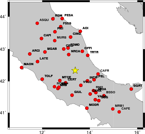
The focal mechanism was determined using broadband seismic waveforms. The location of the event and the and stations used for the waveform inversion are shown in the next figure.
|
|
|
|
The program wvfgrd96 was used with good traces observed at short distance to determine the focal mechanism, depth and seismic moment. This technique requires a high quality signal and well determined velocity model for the Green functions. To the extent that these are the quality data, this type of mechanism should be preferred over the radiation pattern technique which requires the separate step of defining the pressure and tension quadrants and the correct strike.
The observed and predicted traces are filtered using the following gsac commands:
hp c 0.02 n 3
lp c 0.10 n 3
The results of this grid search from 0.5 to 19 km depth are as follow:
           DEPTH  STK   DIP  RAKE   MW    FIT
WVFGRD96    0.5   150    50    90   3.94 0.2565
WVFGRD96    1.0   290    55    30   3.88 0.2016
WVFGRD96    2.0   325    40   -95   4.09 0.2506
WVFGRD96    3.0   130    75    70   4.12 0.2577
WVFGRD96    4.0   135    75    70   4.14 0.3102
WVFGRD96    5.0   140    75    70   4.16 0.3383
WVFGRD96    6.0   200    30   -25   4.15 0.3504
WVFGRD96    7.0   200    30   -30   4.17 0.3653
WVFGRD96    8.0   190    30   -40   4.25 0.3790
WVFGRD96    9.0   190    30   -40   4.27 0.3866
WVFGRD96   10.0   190    35   -40   4.28 0.3876
WVFGRD96   11.0   185    35   -45   4.29 0.3860
WVFGRD96   12.0   180    35   -50   4.30 0.3805
WVFGRD96   13.0   185    40   -40   4.31 0.3725
WVFGRD96   14.0   180    45   -45   4.33 0.3654
WVFGRD96   15.0   180    50   -40   4.34 0.3587
WVFGRD96   16.0   185    55   -30   4.35 0.3513
WVFGRD96   17.0   180    55   -40   4.36 0.3437
WVFGRD96   18.0   175    55   -45   4.37 0.3367
WVFGRD96   19.0   175    55   -45   4.38 0.3310
WVFGRD96   20.0   175    55   -45   4.39 0.3243
WVFGRD96   21.0   175    60   -45   4.41 0.3213
WVFGRD96   22.0   175    60   -45   4.42 0.3153
WVFGRD96   23.0   175    60   -45   4.43 0.3084
WVFGRD96   24.0   180    60   -40   4.43 0.3008
WVFGRD96   25.0   180    60   -40   4.44 0.2935
WVFGRD96   26.0   180    60   -40   4.45 0.2858
WVFGRD96   27.0   180    60   -40   4.45 0.2778
WVFGRD96   28.0     0    50   -40   4.44 0.2699
WVFGRD96   29.0     0    50   -40   4.45 0.2626
The best solution is
WVFGRD96 10.0 190 35 -40 4.28 0.3876
The mechanism correspond to the best fit is
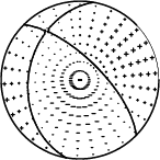
|
|
|
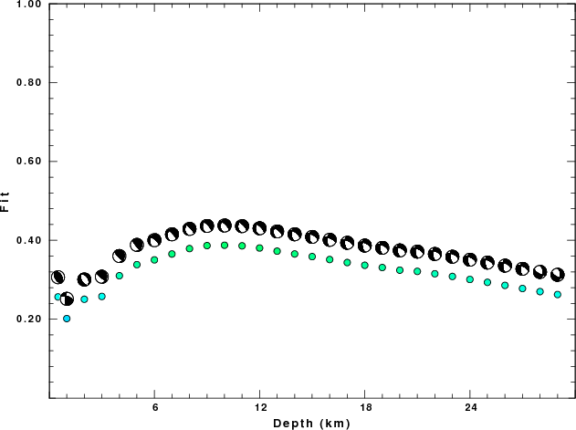
The best fit as a function of depth is given in the following figure:
|
|
|
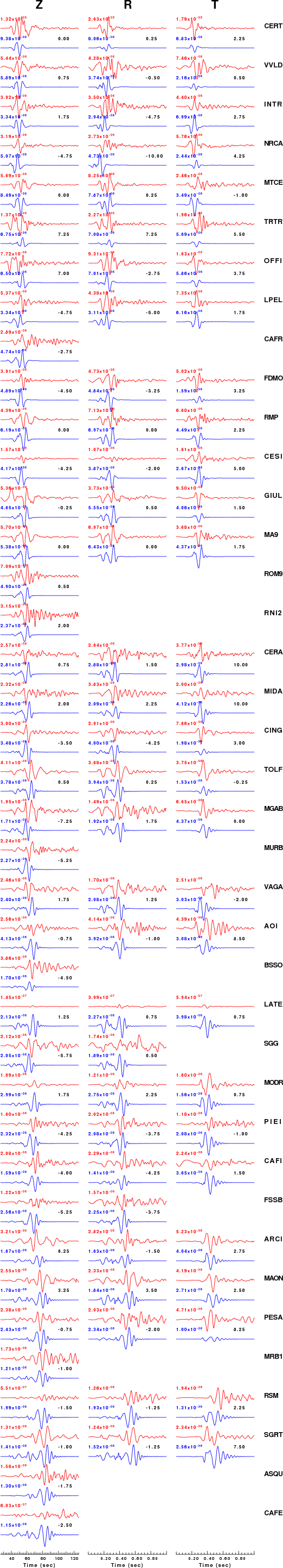
The comparison of the observed and predicted waveforms is given in the next figure. The red traces are the observed and the blue are the predicted. Each observed-predicted component is plotted to the same scale and peak amplitudes are indicated by the numbers to the left of each trace. The number in black at the rightr of each predicted traces it the time shift required for maximum correlation between the observed and predicted traces. This time shift is required because the synthetics are not computed at exactly the same distance as the observed and because the velocity model used in the predictions may not be perfect. A positive time shift indicates that the prediction is too fast and should be delayed to match the observed trace (shift to the right in this figure). A negative value indicates that the prediction is too slow. The bandpass filter used in the processing and for the display was
hp c 0.02 n 3
lp c 0.10 n 3
|
|
|
|
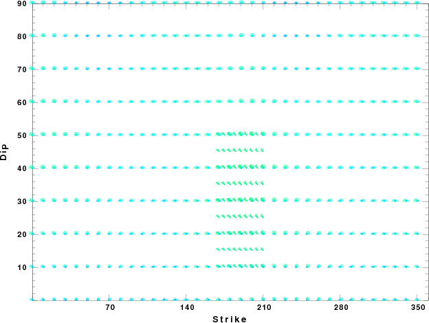
| Focal mechanism sensitivity at the preferred depth. The red color indicates a very good fit to thewavefroms. Each solution is plotted as a vector at a given value of strike and dip with the angle of the vector representing the rake angle, measured, with respect to the upward vertical (N) in the figure. |
The WUS used for the waveform synthetic seismograms and for the surface wave eigenfunctions and dispersion is as follows:
MODEL.01
Model after     8 iterations
ISOTROPIC
KGS
FLAT EARTH
1-D
CONSTANT VELOCITY
LINE08
LINE09
LINE10
LINE11
      H(KM)   VP(KM/S)   VS(KM/S) RHO(GM/CC)         QP         QS       ETAP       ETAS      FREFP      FREFS
     1.9000     3.4065     2.0089     2.2150  0.302E-02  0.679E-02   0.00       0.00       1.00       1.00
     6.1000     5.5445     3.2953     2.6089  0.349E-02  0.784E-02   0.00       0.00       1.00       1.00
    13.0000     6.2708     3.7396     2.7812  0.212E-02  0.476E-02   0.00       0.00       1.00       1.00
    19.0000     6.4075     3.7680     2.8223  0.111E-02  0.249E-02   0.00       0.00       1.00       1.00
     0.0000     7.9000     4.6200     3.2760  0.164E-10  0.370E-10   0.00       0.00       1.00       1.00
Here we tabulate the reasons for not using certain digital data sets
The following stations did not have a valid response files:
DATE=Thu Apr 16 07:11:43 CDT 2009