2008/12/01 10:18:39 35.440 46.109 10.0 5.0 Iran/Iraq Border
2008/12/01 10:18:39 35.440 46.109 10.0 IRAN-IRAQ BORDER REGION M=5.0 (NEIC)
2008/12/01 10:18:41.8 35.45 46.27 15 ML:4.1 18 km East of Marivan, Kordestan Province (IIEES)
Event: 2008-12-01 10:18:38 Lat: 35.3 Lon: 46.2 Depth: 16.0 Mag: 5.0 Type: Mb Origin Author: EMSC-INFO Description: Iran-Iraq border region
USGS Felt map for this earthquake
 SLU Moment Tensor Solution
 2008/12/01 10:18:39 35.440 46.109 10.0 5.0 Iran/Iraq Border

 Best Fitting Double Couple
    Mo = 7.85e+22 dyne-cm
    Mw = 4.53
    Z  = 10 km
     Plane   Strike  Dip  Rake
      NP1      221    87   -50
      NP2      315    40   -175
 Principal Axes:
   Axis    Value   Plunge  Azimuth
     T   7.85e+22     30     280
     N   0.00e+00     40      38
     P  -7.85e+22     36     165


 Moment Tensor: (dyne-cm)
    Component  Value
       Mxx    -4.69e+22
       Mxy     3.37e+21
       Mxz     4.15e+22
       Myy     5.37e+22
       Myz    -4.32e+22
       Mzz    -6.74e+21


                     --------------
                 ----------------------
              ---#######------------------
             #################----------###
           ######################-----#######
          #########################-##########
         #########################---##########
        #########################------#########
        ####   ################---------########
       ##### T ##############------------########
       #####   #############--------------#######
       ###################-----------------######
       ##################------------------######
        ###############---------------------####
        #############-----------------------####
         ###########------------------------###
          ########--------------------------##
           ######-------------   -----------#
             ###-------------- P ----------
              ----------------   ---------
                 ----------------------
                     --------------


 Harvard Convention
 Moment Tensor:
      R          T          F
 -6.74e+21   4.15e+22   4.32e+22
  4.15e+22  -4.69e+22  -3.37e+21
  4.32e+22  -3.37e+21   5.37e+22


Details of the solution is found at

http://www.eas.slu.edu/Earthquake_Center/MECH.IR//index.html
|
      STK = 315
      DIP = 40
     RAKE = -175
       MW = 4.53
       HS = 10
Neither technique provides a good depth constraint. The waveform inversion is affected by the narrow, long period band used for the inversion. The surface-wave technique is affected by the limited azimuthal coverage. However, the gains of the instruments from the different networks seem OK, although there are problems with individual channels. The surface-wave solution is preferred because of the shallower depth.
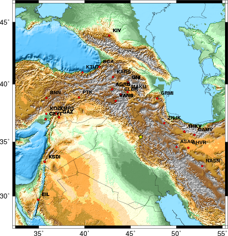
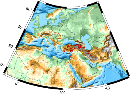
The focal mechanism was determined using broadband seismic waveforms. The location of the event and the and stations used for the waveform inversion are shown in the next figure.
|
|
|
|
The program wvfgrd96 was used with good traces observed at short distance to determine the focal mechanism, depth and seismic moment. This technique requires a high quality signal and well determined velocity model for the Green functions. To the extent that these are the quality data, this type of mechanism should be preferred over the radiation pattern technique which requires the separate step of defining the pressure and tension quadrants and the correct strike.
The observed and predicted traces are filtered using the following gsac commands:
hp c 0.016 n 3
lp c 0.03 n 3
The results of this grid search from 0.5 to 19 km depth are as follow:
           DEPTH  STK   DIP  RAKE   MW    FIT
WVFGRD96    0.5   225    85   -25   4.25 0.3473
WVFGRD96    1.0   225    85   -25   4.27 0.3606
WVFGRD96    2.0   225    85   -25   4.31 0.3868
WVFGRD96    3.0   220    80   -35   4.37 0.4087
WVFGRD96    4.0   220    75   -35   4.39 0.4282
WVFGRD96    5.0   220    75   -35   4.42 0.4426
WVFGRD96    6.0   220    75   -35   4.43 0.4498
WVFGRD96    7.0   220    75   -30   4.44 0.4499
WVFGRD96    8.0   215    70   -40   4.49 0.4624
WVFGRD96    9.0   215    70   -40   4.50 0.4545
WVFGRD96   10.0   220    75   -30   4.48 0.4443
WVFGRD96   11.0   225    85   -25   4.47 0.4329
WVFGRD96   12.0   230    70    30   4.49 0.4339
WVFGRD96   13.0   230    70    30   4.49 0.4373
WVFGRD96   14.0   230    70    30   4.50 0.4412
WVFGRD96   15.0   230    70    30   4.50 0.4440
WVFGRD96   16.0   230    70    25   4.50 0.4479
WVFGRD96   17.0   230    70    25   4.51 0.4527
WVFGRD96   18.0   230    70    25   4.51 0.4567
WVFGRD96   19.0   230    70    25   4.52 0.4605
WVFGRD96   20.0   230    70    25   4.52 0.4635
WVFGRD96   21.0   230    70    25   4.53 0.4648
WVFGRD96   22.0   230    70    25   4.53 0.4661
WVFGRD96   23.0   230    70    20   4.54 0.4668
WVFGRD96   24.0   230    70    20   4.54 0.4677
WVFGRD96   25.0   230    70    20   4.55 0.4683
WVFGRD96   26.0   230    70    20   4.55 0.4685
WVFGRD96   27.0   230    70    20   4.55 0.4689
WVFGRD96   28.0   225    75    15   4.59 0.4693
WVFGRD96   29.0   225    75    15   4.59 0.4694
WVFGRD96   30.0   225    75    15   4.60 0.4696
WVFGRD96   31.0   225    75    15   4.60 0.4687
WVFGRD96   32.0   225    75    15   4.61 0.4678
WVFGRD96   33.0   225    75    15   4.61 0.4660
WVFGRD96   34.0   225    75    15   4.62 0.4640
WVFGRD96   35.0   225    75    15   4.62 0.4620
WVFGRD96   36.0   225    75    15   4.63 0.4592
WVFGRD96   37.0   225    75    15   4.63 0.4558
WVFGRD96   38.0   225    75    15   4.64 0.4527
WVFGRD96   39.0   225    75    15   4.65 0.4484
WVFGRD96   40.0   225    70    20   4.71 0.4384
WVFGRD96   41.0   225    75    20   4.71 0.4351
WVFGRD96   42.0   225    75    20   4.71 0.4313
WVFGRD96   43.0   225    75    20   4.72 0.4269
WVFGRD96   44.0   225    75    15   4.73 0.4226
WVFGRD96   45.0   225    75    15   4.73 0.4184
WVFGRD96   46.0   225    75    15   4.74 0.4137
WVFGRD96   47.0   225    75    15   4.74 0.4086
WVFGRD96   48.0   225    75    15   4.74 0.4034
WVFGRD96   49.0   225    75    15   4.74 0.3979
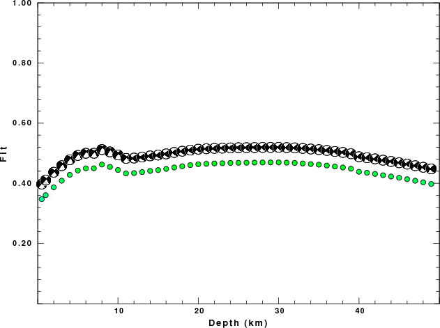
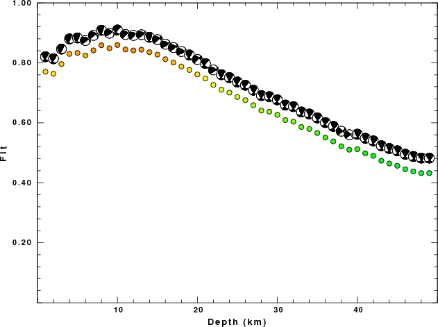
The best solution is
WVFGRD96 30.0 225 75 15 4.60 0.4696
The mechanism correspond to the best fit is
|
|
|
The best fit as a function of depth is given in the following figure:
|
|
|
The comparison of the observed and predicted waveforms is given in the next figure. The red traces are the observed and the blue are the predicted. Each observed-predicted componnet is plotted to the same scale and peak amplitudes are indicated by the numbers to the left of each trace. The number in black at the rightr of each predicted traces it the time shift required for maximum correlation between the observed and predicted traces. This time shift is required because the synthetics are not computed at exactly the same distance as the observed and because the velocity model used in the predictions may not be perfect. A positive time shift indicates that the prediction is too fast and should be delayed to match the observed trace (shift to the right in this figure). A negative value indicates that the prediction is too slow. The bandpass filter used in the processing and for the display was
hp c 0.016 n 3
lp c 0.03 n 3
|
|
|
|
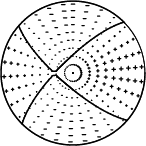
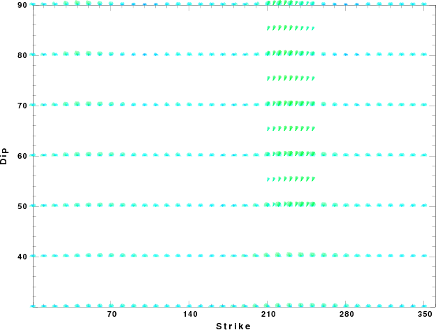
| Focal mechanism sensitivity at the preferred depth. The red color indicates a very good fit to thewavefroms. Each solution is plotted as a vector at a given value of strike and dip with the angle of the vector representing the rake angle, measured, with respect to the upward vertical (N) in the figure. |
The following figure shows the stations used in the grid search for the best focal mechanism to fit the surface-wave spectral amplitudes of the Love and Rayleigh waves.
|
|
|
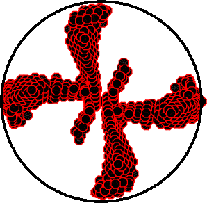
The surface-wave determined focal mechanism is shown here.
  NODAL PLANES


  STK=     221.14
  DIP=      86.78
 RAKE=     -50.10

             OR

  STK=     314.98
  DIP=      40.01
 RAKE=    -174.99


DEPTH = 10.0 km

Mw = 4.53
Best Fit 0.8593 - P-T axis plot gives solutions with FIT greater than FIT90
 |
The P-wave first motion data for focal mechanism studies are as follow:
Sta Az(deg) Dist(km) First motion
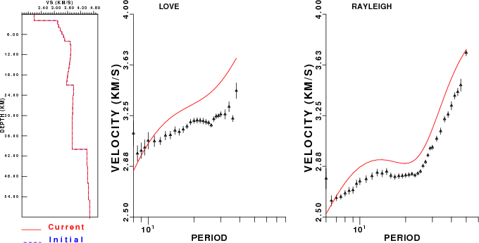
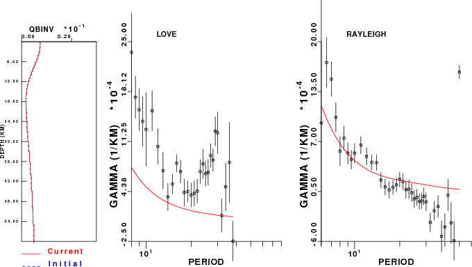
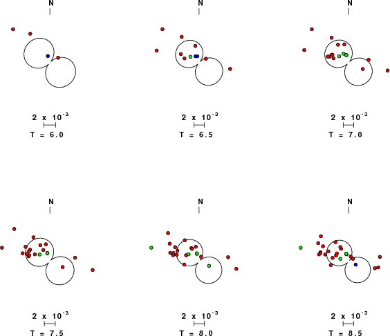
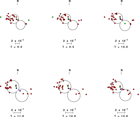
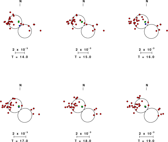
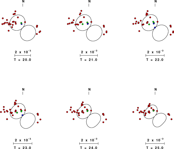
Surface wave analysis was performed using codes from Computer Programs in Seismology, specifically the multiple filter analysis program do_mft and the surface-wave radiation pattern search program srfgrd96.
Digital data were collected, instrument response removed and traces converted
to Z, R an T components. Multiple filter analysis was applied to the Z and T traces to obtain the Rayleigh- and Love-wave spectral amplitudes, respectively.
These were input to the search program which examined all depths between 1 and 25 km
and all possible mechanisms.
|
|
|
|
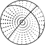
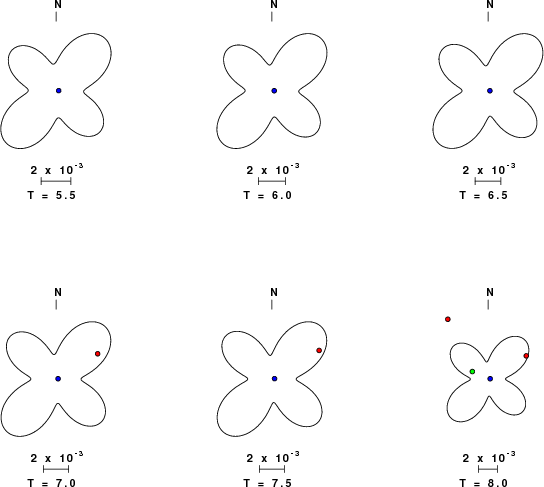
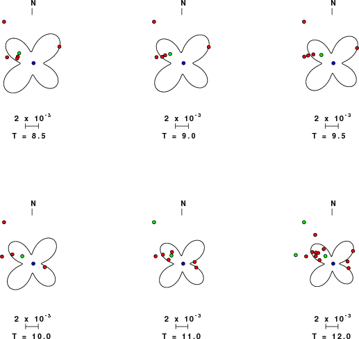
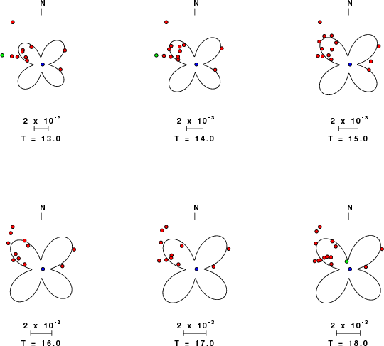
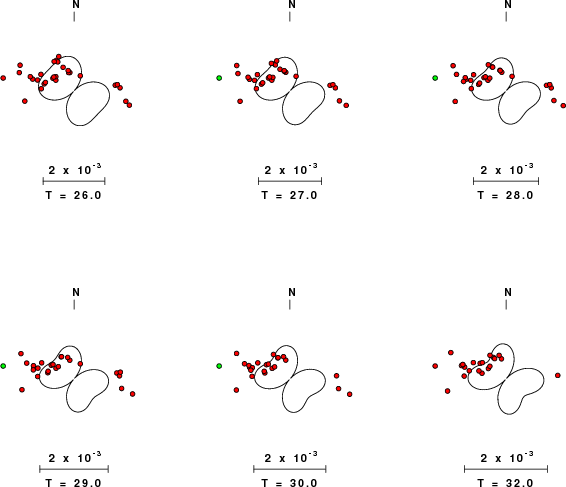
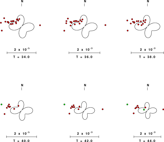
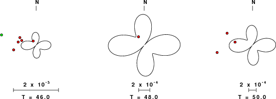
| Pressure-tension axis trends. Since the surface-wave spectra search does not distinguish between P and T axes and since there is a 180 ambiguity in strike, all possible P and T axes are plotted. First motion data and waveforms will be used to select the preferred mechanism. The purpose of this plot is to provide an idea of the possible range of solutions. The P and T-axes for all mechanisms with goodness of fit greater than 0.9 FITMAX (above) are plotted here. |
|
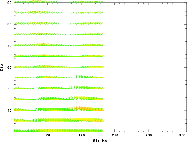
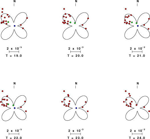
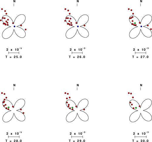
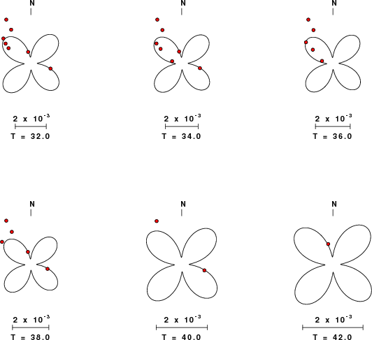
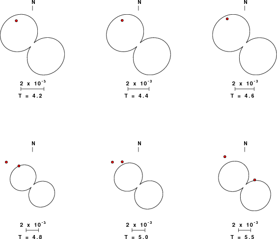
| Focal mechanism sensitivity at the preferred depth. The red color indicates a very good fit to the Love and Rayleigh wave radiation patterns. Each solution is plotted as a vector at a given value of strike and dip with the angle of the vector representing the rake angle, measured, with respect to the upward vertical (N) in the figure. Because of the symmetry of the spectral amplitude rediation patterns, only strikes from 0-180 degrees are sampled. |
The distribution of broadband stations with azimuth and distance is
Sta Az(deg)    Dist(km)
ZNJK	   59	  269
CUKT	  312	  301
ASAO	  104	  371
GRMI	   22	  406
VANB	  326	  426
THKV	   82	  435
MAKU	  344	  452
CLDR	  335	  455
CHTH	   82	  457
GHVR	  101	  485
DAMV	   86	  532
AGRB	  330	  535
GNI	  347	  536
KARS	  336	  632
NASN	  114	  684
PTK	  305	  709
BCA	  331	  773
GAZ	  286	  822
KTUT	  320	  829
KMRS	  288	  856
MERS	  283	  938
CEYT	  284	  947
KOZT	  287	  949
BNN	  296	  986
KIV	  344	  990
KSDI	  258	  993
KVT	  308	 1079
EREN	  274	 1082
CORM	  301	 1138
CANT	  301	 1236
KONT	  287	 1258
LOD	  297	 1275
SHUT	  289	 1425
ELL	  280	 1464
Since the analysis of the surface-wave radiation patterns uses only spectral amplitudes and because the surfave-wave radiation patterns have a 180 degree symmetry, each surface-wave solution consists of four possible focal mechanisms corresponding to the interchange of the P- and T-axes and a roation of the mechanism by 180 degrees. To select one mechanism, P-wave first motion can be used. This was not possible in this case because all the P-wave first motions were emergent ( a feature of the P-wave wave takeoff angle, the station location and the mechanism). The other way to select among the mechanisms is to compute forward synthetics and compare the observed and predicted waveforms.
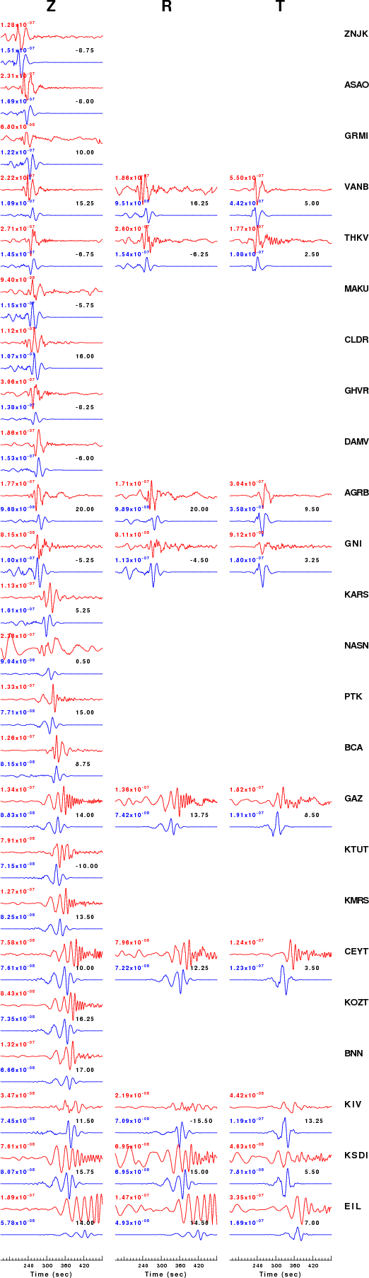
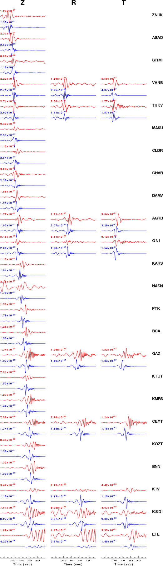
The fits to the waveforms with the given mechanism are show below:
|
This figure shows the fit to the three components of motion (Z - vertical, R-radial and T - transverse). For each station and component, the observed traces is shown in red and the model predicted trace in blue. The traces represent filtered ground velocity in units of meters/sec (the peak value is printed adjacent to each trace; each pair of traces to plotted to the same scale to emphasize the difference in levels). Both synthetic and observed traces have been filtered using the SAC commands:
hp c 0.016 n 3
lp c 0.03 n 3
|
|
The WUS used for the waveform synthetic seismograms and for the surface wave eigenfunctions and dispersion is as follows:
MODEL.01
Model after     8 iterations
ISOTROPIC
KGS
FLAT EARTH
1-D
CONSTANT VELOCITY
LINE08
LINE09
LINE10
LINE11
      H(KM)   VP(KM/S)   VS(KM/S) RHO(GM/CC)         QP         QS       ETAP       ETAS      FREFP      FREFS
     1.9000     3.4065     2.0089     2.2150  0.302E-02  0.679E-02   0.00       0.00       1.00       1.00
     6.1000     5.5445     3.2953     2.6089  0.349E-02  0.784E-02   0.00       0.00       1.00       1.00
    13.0000     6.2708     3.7396     2.7812  0.212E-02  0.476E-02   0.00       0.00       1.00       1.00
    19.0000     6.4075     3.7680     2.8223  0.111E-02  0.249E-02   0.00       0.00       1.00       1.00
     0.0000     7.9000     4.6200     3.2760  0.164E-10  0.370E-10   0.00       0.00       1.00       1.00
Here we tabulate the reasons for not using certain digital data sets