2007/06/18 14:29:54 34.48N 50.84E 42 5.8 Iran
USGS Felt map for this earthquake
USGS Felt reports page for Iran
 SLU Moment Tensor Solution
 2007/06/18 14:29:54 34.48N 50.84E 42 5.8 Iran

 Best Fitting Double Couple
    Mo = 1.43e+24 dyne-cm
    Mw = 5.37
    Z  = 16 km
     Plane   Strike  Dip  Rake
      NP1      148    61   118
      NP2      280    40    50
 Principal Axes:
   Axis    Value   Plunge  Azimuth
     T   1.43e+24     63     105
     N   0.00e+00     24     313
     P  -1.43e+24     11     218


 Moment Tensor: (dyne-cm)
    Component  Value
       Mxx    -8.44e+23
       Mxy    -7.39e+23
       Mxz     6.50e+22
       Myy    -2.34e+23
       Myz     7.26e+23
       Mzz     1.08e+24


                     --------------
                 ----------------------
              ##--------------------------
             ###---------------------------
           #####----###########--------------
          #####-#####################---------
         ###-----#######################-------
        ##-------#########################------
        ----------##########################----
       -----------############################---
       ------------##############   ###########--
       -------------############# T ############-
       --------------############   ############-
        --------------##########################
        ---------------#########################
         ----------------######################
          -----------------###################
           ---   -----------#################
             - P --------------############
                 -----------------########
                 ----------------------
                     --------------


 Harvard Convention
 Moment Tensor:
      R          T          F
  1.08e+24   6.50e+22  -7.26e+23
  6.50e+22  -8.44e+23   7.39e+23
 -7.26e+23   7.39e+23  -2.34e+23


Details of the solution is found at

http://www.eas.slu.edu/Earthquake_Center/MECH.IR/20070618142954/index.html
|
      STK = 280
      DIP = 40
     RAKE = 50
       MW = 5.37
       HS = 16
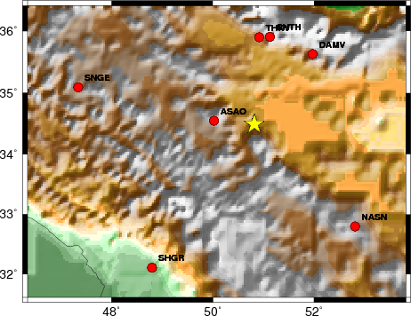
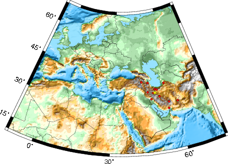
The focal mechanism was determined using broadband seismic waveforms. The location of the event and the and stations used for the waveform inversion are shown in the next figure.
|
|
|
|
The program wvfgrd96 was used with good traces observed at short distance to determine the focal mechanism, depth and seismic moment. This technique requires a high quality signal and well determined velocity model for the Green functions. To the extent that these are the quality data, this type of mechanism should be preferred over the radiation pattern technique which requires the separate step of defining the pressure and tension quadrants and the correct strike.
The observed and predicted traces are filtered using the following gsac commands:
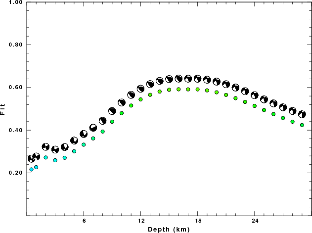
hp c 0.02 n 3
lp c 0.10 n 3
The results of this grid search from 0.5 to 19 km depth are as follow:
           DEPTH  STK   DIP  RAKE   MW    FIT
WVFGRD96    0.5    60    80   -10   4.82 0.2166
WVFGRD96    1.0    60    85    -5   4.86 0.2270
WVFGRD96    2.0    65    90    -5   4.97 0.2724
WVFGRD96    3.0    65    85   -15   5.03 0.2594
WVFGRD96    4.0    60    45   -15   5.09 0.2712
WVFGRD96    5.0    60    45   -15   5.11 0.3017
WVFGRD96    6.0    65    45   -10   5.12 0.3324
WVFGRD96    7.0    65    85   -60   5.14 0.3617
WVFGRD96    8.0   265    30    30   5.21 0.3939
WVFGRD96    9.0   275    30    45   5.24 0.4398
WVFGRD96   10.0   270    35    40   5.27 0.4798
WVFGRD96   11.0   280    35    50   5.29 0.5154
WVFGRD96   12.0   275    40    50   5.32 0.5441
WVFGRD96   13.0   280    40    50   5.33 0.5657
WVFGRD96   14.0   280    40    50   5.35 0.5808
WVFGRD96   15.0   280    40    50   5.36 0.5893
WVFGRD96   16.0   280    40    50   5.37 0.5915
WVFGRD96   17.0   250    55     5   5.41 0.5912
WVFGRD96   18.0   250    55     0   5.42 0.5910
WVFGRD96   19.0   250    55     0   5.44 0.5864
WVFGRD96   20.0   250    55    -5   5.44 0.5774
WVFGRD96   21.0   250    55     0   5.46 0.5653
WVFGRD96   22.0   250    55     0   5.47 0.5497
WVFGRD96   23.0   250    50    -5   5.46 0.5325
WVFGRD96   24.0   250    50    -5   5.47 0.5138
WVFGRD96   25.0   250    50    -5   5.47 0.4943
WVFGRD96   26.0   250    50   -10   5.48 0.4755
WVFGRD96   27.0   250    50   -10   5.48 0.4572
WVFGRD96   28.0   250    50   -15   5.48 0.4401
WVFGRD96   29.0   250    50   -15   5.49 0.4244
The best solution is
WVFGRD96 16.0 280 40 50 5.37 0.5915
The mechanism correspond to the best fit is
|
|
|
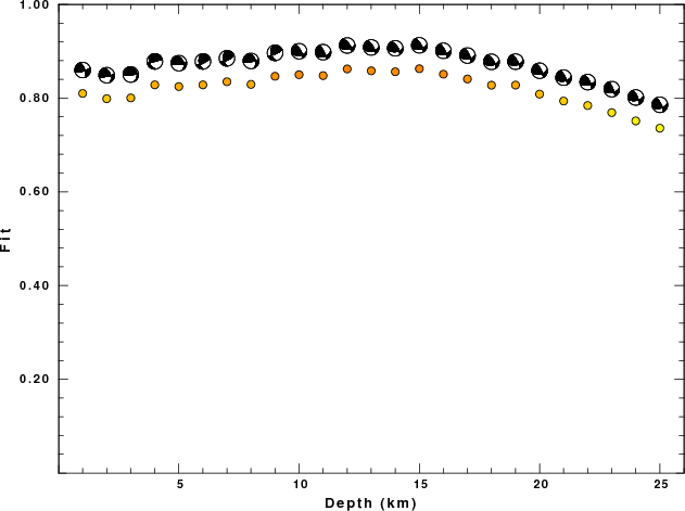
The best fit as a function of depth is given in the following figure:
|
|
|
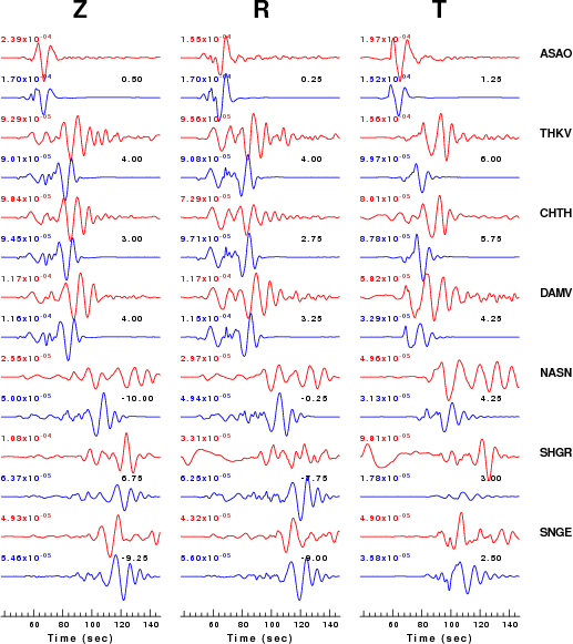
The comparison of the observed and predicted waveforms is given in the next figure. The red traces are the observed and the blue are the predicted. Each observed-predicted componnet is plotted to the same scale and peak amplitudes are indicated by the numbers to the left of each trace. The number in black at the rightr of each predicted traces it the time shift required for maximum correlation between the observed and predicted traces. This time shift is required because the synthetics are not computed at exactly the same distance as the observed and because the velocity model used in the predictions may not be perfect. A positive time shift indicates that the prediction is too fast and should be delayed to match the observed trace (shift to the right in this figure). A negative value indicates that the prediction is too slow. The bandpass filter used in the processing and for the display was
hp c 0.02 n 3
lp c 0.10 n 3
|
|
|
|
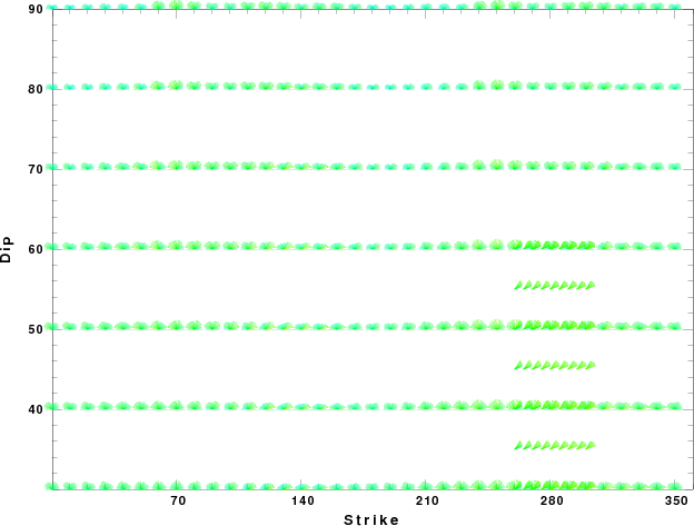
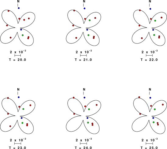
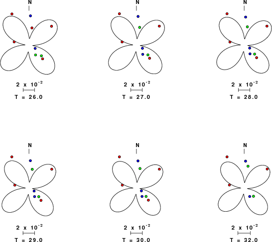
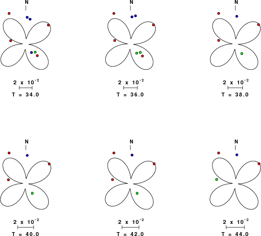
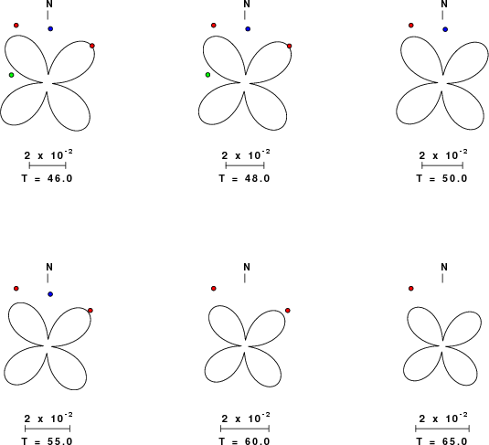
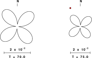
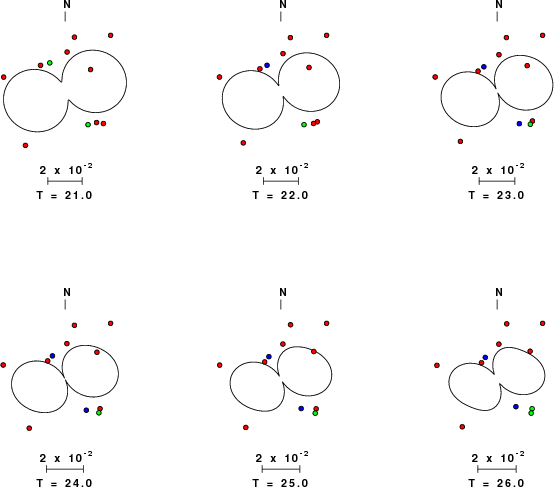
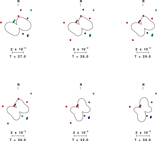
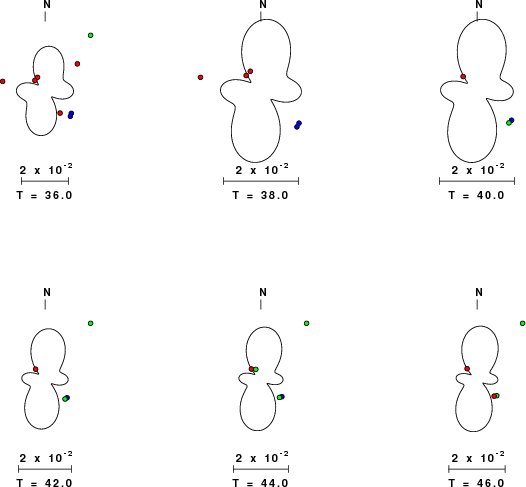
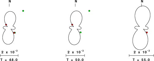
| Focal mechanism sensitivity at the preferred depth. The red color indicates a very good fit to thewavefroms. Each solution is plotted as a vector at a given value of strike and dip with the angle of the vector representing the rake angle, measured, with respect to the upward vertical (N) in the figure. |
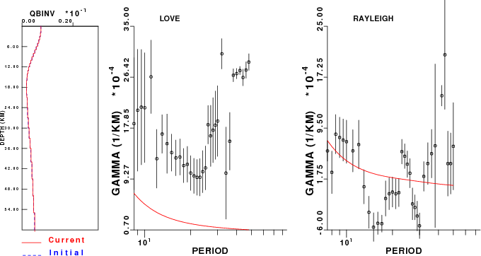
The following figure shows the stations used in the grid search for the best focal mechanism to fit the surface-wave spectral amplitudes of the Love and Rayleigh waves.
|
|
|
The surface-wave determined focal mechanism is shown here.
  NODAL PLANES


  STK=     124.30
  DIP=      62.97
 RAKE=     127.46

             OR

  STK=     244.98
  DIP=      45.00
 RAKE=      40.00


DEPTH = 12.0 km

Mw = 5.44
Best Fit 0.8623 - P-T axis plot gives solutions with FIT greater than FIT90
 |
The P-wave first motion data for focal mechanism studies are as follow:
Sta Az(deg) Dist(km) First motion
Surface wave analysis was performed using codes from Computer Programs in Seismology, specifically the multiple filter analysis program do_mft and the surface-wave radiation pattern search program srfgrd96.
Digital data were collected, instrument response removed and traces converted
to Z, R an T components. Multiple filter analysis was applied to the Z and T traces to obtain the Rayleigh- and Love-wave spectral amplitudes, respectively.
These were input to the search program which examined all depths between 1 and 25 km
and all possible mechanisms.
|
|
|
|
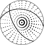
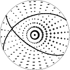
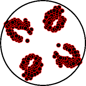
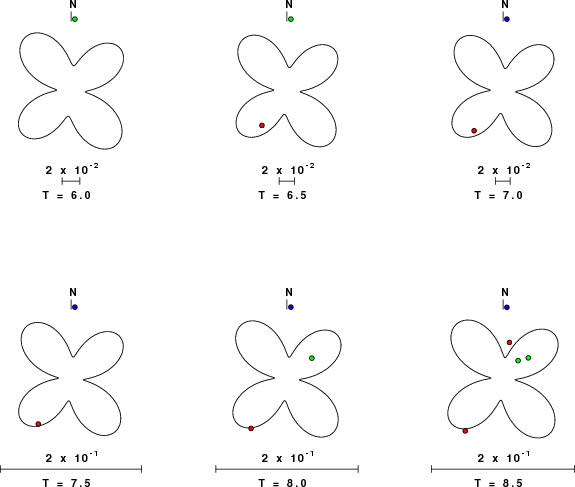
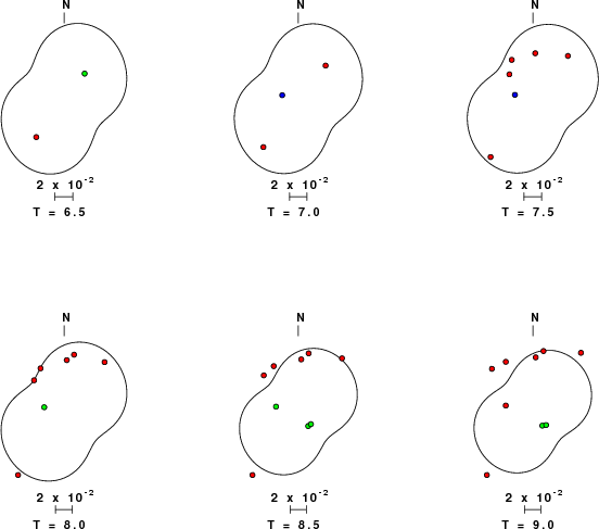
| Pressure-tension axis trends. Since the surface-wave spectra search does not distinguish between P and T axes and since there is a 180 ambiguity in strike, all possible P and T axes are plotted. First motion data and waveforms will be used to select the preferred mechanism. The purpose of this plot is to provide an idea of the possible range of solutions. The P and T-axes for all mechanisms with goodness of fit greater than 0.9 FITMAX (above) are plotted here. |
|
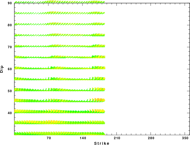
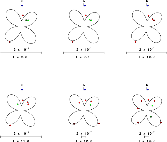
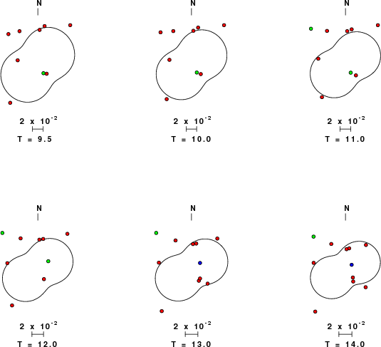
| Focal mechanism sensitivity at the preferred depth. The red color indicates a very good fit to the Love and Rayleigh wave radiation patterns. Each solution is plotted as a vector at a given value of strike and dip with the angle of the vector representing the rake angle, measured, with respect to the upward vertical (N) in the figure. Because of the symmetry of the spectral amplitude rediation patterns, only strikes from 0-180 degrees are sampled. |
The distribution of broadband stations with azimuth and distance is
Sta Az(deg)    Dist(km)
ASAO	  275	   73
THKV	    3	  157
CHTH	   10	  160
DAMV	   39	  164
NASN	  135	  263
SHGR	  216	  324
SNGE	  283	  325
GRMI	  332	  547
MRVT	   50	  590
KRBR	  130	  750
MAKU	  316	  768
BNDS	  146	  939
ZHSF	  117	 1085
Since the analysis of the surface-wave radiation patterns uses only spectral amplitudes and because the surfave-wave radiation patterns have a 180 degree symmetry, each surface-wave solution consists of four possible focal mechanisms corresponding to the interchange of the P- and T-axes and a roation of the mechanism by 180 degrees. To select one mechanism, P-wave first motion can be used. This was not possible in this case because all the P-wave first motions were emergent ( a feature of the P-wave wave takeoff angle, the station location and the mechanism). The other way to select among the mechanisms is to compute forward synthetics and compare the observed and predicted waveforms.
The fits to the waveforms with the given mechanism are show below:
|
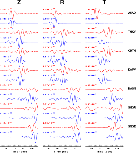
This figure shows the fit to the three components of motion (Z - vertical, R-radial and T - transverse). For each station and component, the observed traces is shown in red and the model predicted trace in blue. The traces represent filtered ground velocity in units of meters/sec (the peak value is printed adjacent to each trace; each pair of traces to plotted to the same scale to emphasize the difference in levels). Both synthetic and observed traces have been filtered using the SAC commands:
hp c 0.02 n 3
lp c 0.10 n 3
|
|
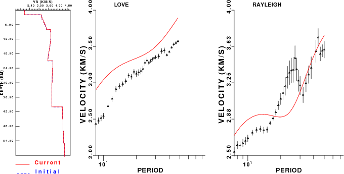
The WUS used for the waveform synthetic seismograms and for the surface wave eigenfunctions and dispersion is as follows:
MODEL.01
Model after     8 iterations
ISOTROPIC
KGS
FLAT EARTH
1-D
CONSTANT VELOCITY
LINE08
LINE09
LINE10
LINE11
      H(KM)   VP(KM/S)   VS(KM/S) RHO(GM/CC)         QP         QS       ETAP       ETAS      FREFP      FREFS
     1.9000     3.4065     2.0089     2.2150  0.302E-02  0.679E-02   0.00       0.00       1.00       1.00
     6.1000     5.5445     3.2953     2.6089  0.349E-02  0.784E-02   0.00       0.00       1.00       1.00
    13.0000     6.2708     3.7396     2.7812  0.212E-02  0.476E-02   0.00       0.00       1.00       1.00
    19.0000     6.4075     3.7680     2.8223  0.111E-02  0.249E-02   0.00       0.00       1.00       1.00
     0.0000     7.9000     4.6200     3.2760  0.164E-10  0.370E-10   0.00       0.00       1.00       1.00
Here we tabulate the reasons for not using certain digital data sets