Location
Location ANSS
2023/06/16 16:38:28 46.21 -0.77 10.0 5.0 France
Focal Mechanism
 USGS/SLU Moment Tensor Solution
 ENS  2023/06/16 16:38:28:8  46.21   -0.77  10.0 5.0 France

 Stations used:
   C4.CERNS CH.BRANT CH.COLLE CH.GIMEL CH.LASAR CH.MESRY
   CH.PERON CH.SALEV CH.VINZL FR.ABJF FR.ATE FR.BALS FR.BANN
   FR.BARI FR.BEGF FR.BESN FR.BIMF FR.BORF FR.BOUC FR.BOUF
   FR.BRGF FR.BSCF FR.CHIF FR.CHLF FR.CLAF FR.CLF FR.COLF
   FR.CRAS FR.CRNF FR.CSCF FR.CURIE FR.DAUF FR.DUNF FR.FAHY
   FR.FILF FR.FNEB FR.FOURG FR.GARF FR.GENF FR.GIZF FR.GNEF
   FR.GOTF FR.GRN FR.GUEF FR.GZNF FR.HRSF FR.IRAF FR.LABF
   FR.LATF FR.LEUC FR.LGIF FR.LOCF FR.LOUF FR.LRVF FR.MERIC
   FR.MLS FR.MTNF FR.OG35 FR.OGCB FR.OGCC FR.OGCN FR.OGDF
   FR.OGGL FR.OGMY FR.OGS1 FR.OGSM FR.OLIV FR.ORDF FR.OSSF
   FR.PAND FR.PYHE FR.RESF FR.REST FR.REYF FR.RIAF FR.RIVEL
   FR.RUFF FR.SALF FR.SAUF FR.SDOF FR.SGSF FR.SLVF FR.SOMF
   FR.SRNF FR.SROF FR.TERF FR.TSDF FR.URDF FR.VALC FR.VALM
   FR.VERF FR.VIEF GB.JSA MT.AVM MT.AVP XP.FR01A

 Filtering commands used:
   cut o DIST/3.3 -40 o DIST/3.3 +50
   rtr
   taper w 0.1
   hp c 0.03 n 3
   lp c 0.06 n 3

 Best Fitting Double Couple
  Mo = 1.80e+23 dyne-cm
  Mw = 4.77
  Z  = 11 km
  Plane   Strike  Dip  Rake
   NP1       87    85   -160
   NP2      355    70    -5
  Principal Axes:
   Axis    Value   Plunge  Azimuth
    T   1.80e+23     11     219
    N   0.00e+00     69      99
    P  -1.80e+23     17     313

 Moment Tensor: (dyne-cm)
    Component   Value
       Mxx     2.93e+22
       Mxy     1.67e+23
       Mxz    -6.00e+22
       Myy    -1.92e+22
       Myz     1.73e+22
       Mzz    -1.01e+22


                     ------########
                 -----------###########
              ---------------#############
             -   -------------#############
           --- P --------------##############
          ----   --------------###############
         -----------------------###############
        ------------------------################
        -------------------------###############
       --------------------------################
       --------------------------##############--
       -------------------------#----------------
       ##########################----------------
        #########################---------------
        #########################---------------
         ########################--------------
          #######################-------------
           ###   ################------------
             # T ###############-----------
                 ###############----------
                 ##############--------
                     #########-----


 Global CMT Convention Moment Tensor:
      R          T          P
 -1.01e+22  -6.00e+22  -1.73e+22
 -6.00e+22   2.93e+22  -1.67e+23
 -1.73e+22  -1.67e+23  -1.92e+22


Details of the solution is found at

http://www.eas.slu.edu/eqc/eqc_mt/MECH.NA/20230616163828/index.html
|
Preferred Solution
The preferred solution from an analysis of the surface-wave spectral amplitude radiation pattern, waveform inversion and first motion observations is
      STK = -5
      DIP = 70
     RAKE = -5
       MW = 4.77
       HS = 11.0
The NDK file is 20230616163828.ndk
The waveform inversion is preferred.
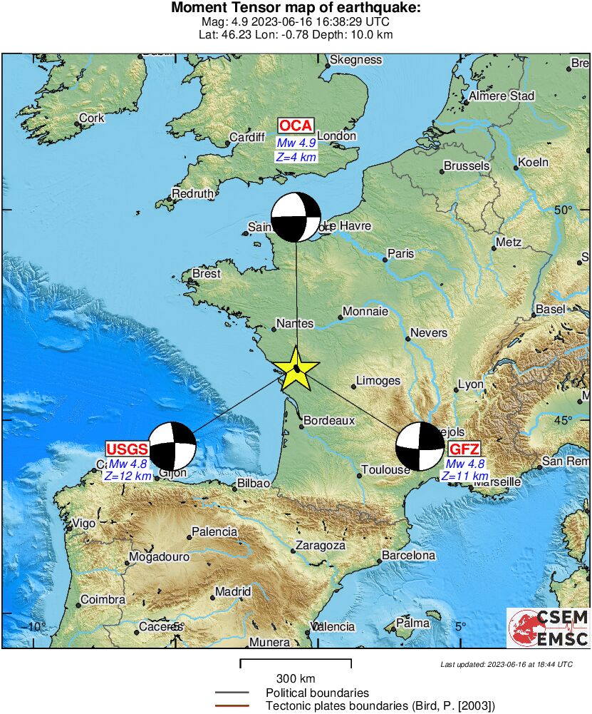
Moment Tensor Comparison
The following compares this source inversion to others
| WVFGRD |
USGSW |
OTHER |
 USGS/SLU Moment Tensor Solution
 ENS  2023/06/16 16:38:28:8  46.21   -0.77  10.0 5.0 France

 Stations used:
   C4.CERNS CH.BRANT CH.COLLE CH.GIMEL CH.LASAR CH.MESRY
   CH.PERON CH.SALEV CH.VINZL FR.ABJF FR.ATE FR.BALS FR.BANN
   FR.BARI FR.BEGF FR.BESN FR.BIMF FR.BORF FR.BOUC FR.BOUF
   FR.BRGF FR.BSCF FR.CHIF FR.CHLF FR.CLAF FR.CLF FR.COLF
   FR.CRAS FR.CRNF FR.CSCF FR.CURIE FR.DAUF FR.DUNF FR.FAHY
   FR.FILF FR.FNEB FR.FOURG FR.GARF FR.GENF FR.GIZF FR.GNEF
   FR.GOTF FR.GRN FR.GUEF FR.GZNF FR.HRSF FR.IRAF FR.LABF
   FR.LATF FR.LEUC FR.LGIF FR.LOCF FR.LOUF FR.LRVF FR.MERIC
   FR.MLS FR.MTNF FR.OG35 FR.OGCB FR.OGCC FR.OGCN FR.OGDF
   FR.OGGL FR.OGMY FR.OGS1 FR.OGSM FR.OLIV FR.ORDF FR.OSSF
   FR.PAND FR.PYHE FR.RESF FR.REST FR.REYF FR.RIAF FR.RIVEL
   FR.RUFF FR.SALF FR.SAUF FR.SDOF FR.SGSF FR.SLVF FR.SOMF
   FR.SRNF FR.SROF FR.TERF FR.TSDF FR.URDF FR.VALC FR.VALM
   FR.VERF FR.VIEF GB.JSA MT.AVM MT.AVP XP.FR01A

 Filtering commands used:
   cut o DIST/3.3 -40 o DIST/3.3 +50
   rtr
   taper w 0.1
   hp c 0.03 n 3
   lp c 0.06 n 3

 Best Fitting Double Couple
  Mo = 1.80e+23 dyne-cm
  Mw = 4.77
  Z  = 11 km
  Plane   Strike  Dip  Rake
   NP1       87    85   -160
   NP2      355    70    -5
  Principal Axes:
   Axis    Value   Plunge  Azimuth
    T   1.80e+23     11     219
    N   0.00e+00     69      99
    P  -1.80e+23     17     313

 Moment Tensor: (dyne-cm)
    Component   Value
       Mxx     2.93e+22
       Mxy     1.67e+23
       Mxz    -6.00e+22
       Myy    -1.92e+22
       Myz     1.73e+22
       Mzz    -1.01e+22


                     ------########
                 -----------###########
              ---------------#############
             -   -------------#############
           --- P --------------##############
          ----   --------------###############
         -----------------------###############
        ------------------------################
        -------------------------###############
       --------------------------################
       --------------------------##############--
       -------------------------#----------------
       ##########################----------------
        #########################---------------
        #########################---------------
         ########################--------------
          #######################-------------
           ###   ################------------
             # T ###############-----------
                 ###############----------
                 ##############--------
                     #########-----


 Global CMT Convention Moment Tensor:
      R          T          P
 -1.01e+22  -6.00e+22  -1.73e+22
 -6.00e+22   2.93e+22  -1.67e+23
 -1.73e+22  -1.67e+23  -1.92e+22


Details of the solution is found at

http://www.eas.slu.edu/eqc/eqc_mt/MECH.NA/20230616163828/index.html
|
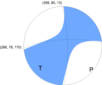
W-phase Moment Tensor (Mww)
Moment 2.271e+16 N-m
Magnitude 4.84 Mww
Depth 11.5 km
Percent DC 68%
Half Duration 0.70 s
Catalog US
Data Source US 1
Contributor US 1

Nodal Planes
Plane Strike Dip Rake
NP1 266 78 170
NP2 359 80 13

Principal Axes
Axis Value Plunge Azimuth
T 2.051e+16 N-m 16 223
N 0.388e+16 N-m 74 36
P -2.440e+16 N-m 2
|
|
Magnitudes
mLg Magnitude
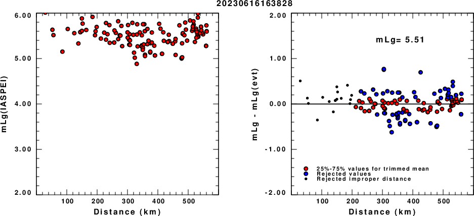
(a) mLg computed using the IASPEI formula; (b) mLg residuals ; the values used for the trimmed mean are indicated.
ML Magnitude
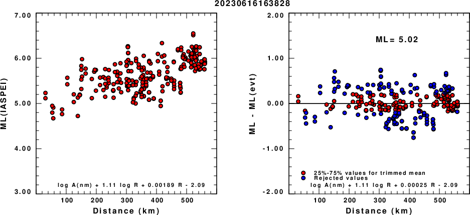
(a) ML computed using the IASPEI formula for Horizontal components; (b) ML residuals computed using a modified IASPEI formula that accounts for path specific attenuation; the values used for the trimmed mean are indicated. The ML relation used for each figure is given at the bottom of each plot.
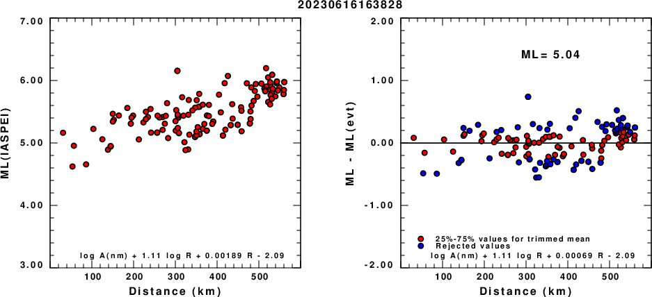
(a) ML computed using the IASPEI formula for Vertical components (research); (b) ML residuals computed using a modified IASPEI formula that accounts for path specific attenuation; the values used for the trimmed mean are indicated. The ML relation used for each figure is given at the bottom of each plot.
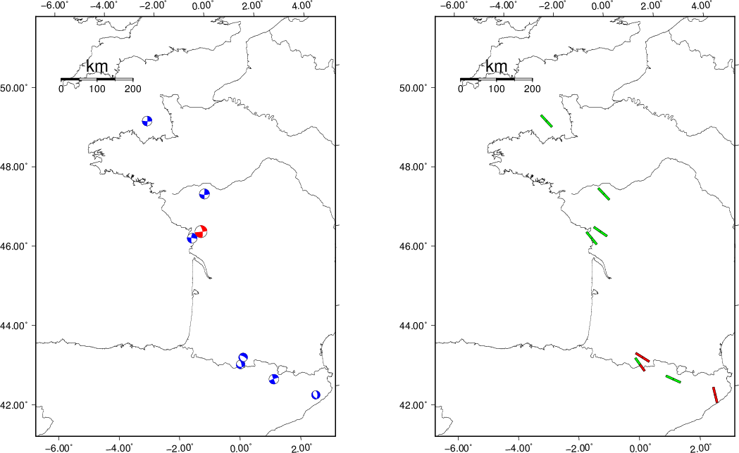
Context
The next figure presents the focal mechanism for this earthquake (red) in the context of other events (blue) in the SLU Moment Tensor Catalog which are within ± 0.5 degrees of the new event. This comparison is shown in the left panel of the figure. The right panel shows the inferred direction of maximum compressive stress and the type of faulting (green is strike-slip, red is normal, blue is thrust; oblique is shown by a combination of colors).
Waveform Inversion using wvfgrd96
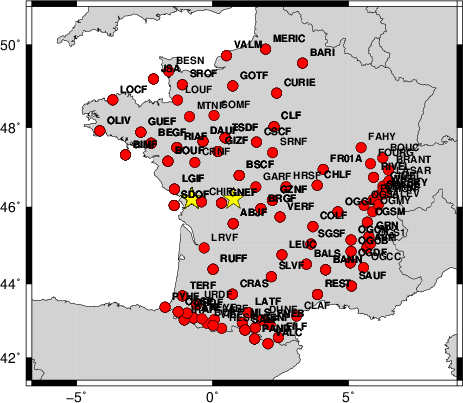
The focal mechanism was determined using broadband seismic waveforms. The location of the event and the
and stations used for the waveform inversion are shown in the next figure.
|
|
Location of broadband stations used for waveform inversion
|
The program wvfgrd96 was used with good traces observed at short distance to determine the focal mechanism, depth and seismic moment. This technique requires a high quality signal and well determined velocity model for the Green functions. To the extent that these are the quality data, this type of mechanism should be preferred over the radiation pattern technique which requires the separate step of defining the pressure and tension quadrants and the correct strike.
The observed and predicted traces are filtered using the following gsac commands:
cut o DIST/3.3 -40 o DIST/3.3 +50
rtr
taper w 0.1
hp c 0.03 n 3
lp c 0.06 n 3
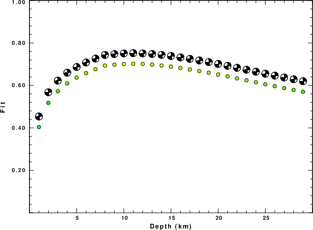
The results of this grid search are as follow:
           DEPTH  STK   DIP  RAKE   MW    FIT
WVFGRD96    1.0    -5    85     0   4.43 0.4039
WVFGRD96    2.0    -5    85    -5   4.53 0.5180
WVFGRD96    3.0    -5    80     0   4.58 0.5726
WVFGRD96    4.0    -5    75     0   4.62 0.6098
WVFGRD96    5.0    -5    75     0   4.65 0.6368
WVFGRD96    6.0    -5    75     0   4.67 0.6580
WVFGRD96    7.0    -5    75     0   4.70 0.6764
WVFGRD96    8.0    -5    70     0   4.73 0.6937
WVFGRD96    9.0    -5    70     0   4.75 0.6978
WVFGRD96   10.0    -5    70    -5   4.76 0.7009
WVFGRD96   11.0    -5    70    -5   4.77 0.7020
WVFGRD96   12.0    -5    70    -5   4.78 0.7010
WVFGRD96   13.0    -5    70    -5   4.79 0.6983
WVFGRD96   14.0    -5    70    -5   4.80 0.6939
WVFGRD96   15.0    -5    70    -5   4.81 0.6887
WVFGRD96   16.0    -5    70    -5   4.82 0.6822
WVFGRD96   17.0    -5    75    -5   4.82 0.6752
WVFGRD96   18.0    -5    75    -5   4.83 0.6679
WVFGRD96   19.0    -5    75    -5   4.84 0.6599
WVFGRD96   20.0    -5    75    -5   4.85 0.6513
WVFGRD96   21.0    -5    75    -5   4.85 0.6424
WVFGRD96   22.0    -5    75    -5   4.86 0.6331
WVFGRD96   23.0    -5    75    -5   4.87 0.6241
WVFGRD96   24.0    -5    75    -5   4.87 0.6148
WVFGRD96   25.0    -5    75    -5   4.88 0.6053
WVFGRD96   26.0    -5    75    -5   4.89 0.5964
WVFGRD96   27.0    -5    75    -5   4.89 0.5876
WVFGRD96   28.0    -5    75    -5   4.90 0.5788
WVFGRD96   29.0    -5    80    -5   4.90 0.5699
The best solution is
WVFGRD96 11.0 -5 70 -5 4.77 0.7020
The mechanism correspond to the best fit is
|
|
Figure 1. Waveform inversion focal mechanism
|
The best fit as a function of depth is given in the following figure:
|
|
Figure 2. Depth sensitivity for waveform mechanism
|
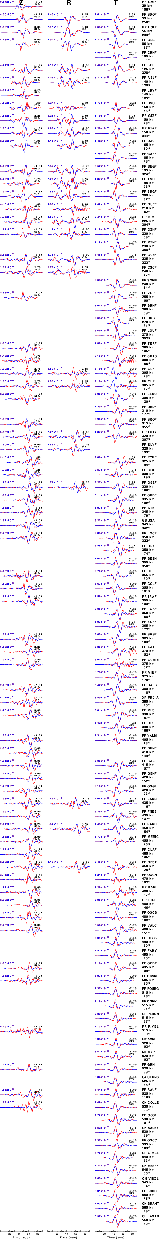
The comparison of the observed and predicted waveforms is given in the next figure. The red traces are the observed and the blue are the predicted.
Each observed-predicted component is plotted to the same scale and peak amplitudes are indicated by the numbers to the left of each trace. A pair of numbers is given in black at the right of each predicted traces. The upper number it the time shift required for maximum correlation between the observed and predicted traces. This time shift is required because the synthetics are not computed at exactly the same distance as the observed and because the velocity model used in the predictions may not be perfect.
A positive time shift indicates that the prediction is too fast and should be delayed to match the observed trace (shift to the right in this figure). A negative value indicates that the prediction is too slow. The lower number gives the percentage of variance reduction to characterize the individual goodness of fit (100% indicates a perfect fit).
The bandpass filter used in the processing and for the display was
cut o DIST/3.3 -40 o DIST/3.3 +50
rtr
taper w 0.1
hp c 0.03 n 3
lp c 0.06 n 3
|
|
Figure 3. Waveform comparison for selected depth. Red: observed; Blue - predicted. The time shift with respect to the model prediction is indicated. The percent of fit is also indicated. The time scale is based on the last trace plotted. It is not used to represent travel time or absolute time, but rather to indicate the number of seconds plotted. If there is not a trace directly above the scale, then a default, meaningless scale is plotted.
|
|
|
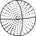
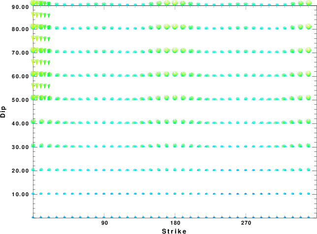
Focal mechanism sensitivity at the preferred depth. The red color indicates a very good fit to thewavefroms.
Each solution is plotted as a vector at a given value of strike and dip with the angle of the vector representing the rake angle, measured, with respect to the upward vertical (N) in the figure.
|
A check on the assumed source location is possible by looking at the time shifts between the observed and predicted traces. The time shifts for waveform matching arise for several reasons:
- The origin time and epicentral distance are incorrect
- The velocity model used for the inversion is incorrect
- The velocity model used to define the P-arrival time is not the
same as the velocity model used for the waveform inversion
(assuming that the initial trace alignment is based on the
P arrival time)
Assuming only a mislocation, the time shifts are fit to a functional form:
Time_shift = A + B cos Azimuth + C Sin Azimuth
The time shifts for this inversion lead to the next figure:
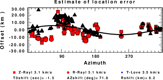
The derived shift in origin time and epicentral coordinates are given at the bottom of the figure.
Discussion
Acknowledgements
Thanks also to the many seismic network operators whose dedication make this effort possible: University of Nevada Reno, University of Alaska, University of Washington, Oregon State University, University of Utah, Montana Bureau of Mines, UC Berkely, Caltech, UC San Diego, Saint Louis University, University of Memphis, Lamont Doherty Earth Observatory, the Oklahoma Geological Survey, TexNet, the Iris stations, the Transportable Array of EarthScope and other networks.
Velocity Model
The WUS.model used for the waveform synthetic seismograms and for the surface wave eigenfunctions and dispersion is as follows:
MODEL.01
Model after     8 iterations
ISOTROPIC
KGS
FLAT EARTH
1-D
CONSTANT VELOCITY
LINE08
LINE09
LINE10
LINE11
      H(KM)   VP(KM/S)   VS(KM/S) RHO(GM/CC)         QP         QS       ETAP       ETAS      FREFP      FREFS
     1.9000     3.4065     2.0089     2.2150  0.302E-02  0.679E-02   0.00       0.00       1.00       1.00
     6.1000     5.5445     3.2953     2.6089  0.349E-02  0.784E-02   0.00       0.00       1.00       1.00
    13.0000     6.2708     3.7396     2.7812  0.212E-02  0.476E-02   0.00       0.00       1.00       1.00
    19.0000     6.4075     3.7680     2.8223  0.111E-02  0.249E-02   0.00       0.00       1.00       1.00
     0.0000     7.9000     4.6200     3.2760  0.164E-10  0.370E-10   0.00       0.00       1.00       1.00
Quality Control
Here we tabulate the reasons for not using certain digital data sets
The following stations did not have a valid response files:
Last Changed Sat Jun 17 16:31:36 CDT 2023