Location

Location ANSS

2023/04/15 22:10:42 45.03 18.38 10.0 4.4 Bosnia

Focal Mechanism

USGS/SLU Moment Tensor Solution ENS 2023/04/15 22:10:42:3 45.03 18.38 10.0 4.4 Bosnia Stations used: AC.BCI BS.BLKB CZ.JAVC HU.BEHE HU.BUD HU.EGYH HU.KOVH HU.MORH HU.SOP HU.TIH IV.SGRT IV.TREM MN.BLY MN.DIVS MN.PDG MN.TIR MN.TRI NI.DST2 NI.VINO OE.ARSA OE.CONA OE.CSNA OE.MOA OE.RONA OE.SOKA OE.VIE OX.ACOM OX.DRE OX.MPRI OX.PRED OX.SABO RO.BANR RO.BZS RO.GZR RO.LOT RO.RMGR RO.SRE RO.SURR SK.MODS Y5.BH02A Y5.BH06A Y5.BH08A Y5.BH09A Y5.BH10A Y5.BH11A Y5.BH12A Y5.BH13A Y5.BH16A Y5.BH18A Y5.BH20A Filtering commands used: cut o DIST/3.3 -40 o DIST/3.3 +50 rtr taper w 0.1 hp c 0.03 n 3 lp c 0.10 n 3 Best Fitting Double Couple Mo = 8.91e+21 dyne-cm Mw = 3.90 Z = 10 km Plane Strike Dip Rake NP1 154 76 154 NP2 250 65 15 Principal Axes: Axis Value Plunge Azimuth T 8.91e+21 28 110 N 0.00e+00 61 308 P -8.91e+21 8 204 Moment Tensor: (dyne-cm) Component Value Mxx -6.58e+21 Mxy -5.41e+21 Mxz -1.49e+20 Myy 4.81e+21 Myz 3.93e+21 Mzz 1.77e+21 -------------- ##-------------------- #####----------------------- ######------------------------ #########------------------------- ##########-------------------------- ############---------------#######---- #############------##################### ##############-######################### ############----########################## #########--------######################### #######-----------######################## #####--------------############### ##### ##-----------------############## T #### #-------------------############# #### --------------------################## --------------------################ --------------------############## --------------------########## ----- ------------######## -- P --------------### ------------- Global CMT Convention Moment Tensor: R T P 1.77e+21 -1.49e+20 -3.93e+21 -1.49e+20 -6.58e+21 5.41e+21 -3.93e+21 5.41e+21 4.81e+21 Details of the solution is found at http://www.eas.slu.edu/eqc/eqc_mt/MECH.NA/20230415221042/index.html

Preferred Solution

The preferred solution from an analysis of the surface-wave spectral amplitude radiation pattern, waveform inversion and first motion observations is

      STK = 250
      DIP = 65
     RAKE = 15
       MW = 3.90
       HS = 10.0

The NDK file is 20230415221042.ndk The waveform inversion is preferred.

Moment Tensor Comparison

The following compares this source inversion to others

WVFGRD

USGS/SLU Moment Tensor Solution ENS 2023/04/15 22:10:42:3 45.03 18.38 10.0 4.4 Bosnia Stations used: AC.BCI BS.BLKB CZ.JAVC HU.BEHE HU.BUD HU.EGYH HU.KOVH HU.MORH HU.SOP HU.TIH IV.SGRT IV.TREM MN.BLY MN.DIVS MN.PDG MN.TIR MN.TRI NI.DST2 NI.VINO OE.ARSA OE.CONA OE.CSNA OE.MOA OE.RONA OE.SOKA OE.VIE OX.ACOM OX.DRE OX.MPRI OX.PRED OX.SABO RO.BANR RO.BZS RO.GZR RO.LOT RO.RMGR RO.SRE RO.SURR SK.MODS Y5.BH02A Y5.BH06A Y5.BH08A Y5.BH09A Y5.BH10A Y5.BH11A Y5.BH12A Y5.BH13A Y5.BH16A Y5.BH18A Y5.BH20A Filtering commands used: cut o DIST/3.3 -40 o DIST/3.3 +50 rtr taper w 0.1 hp c 0.03 n 3 lp c 0.10 n 3 Best Fitting Double Couple Mo = 8.91e+21 dyne-cm Mw = 3.90 Z = 10 km Plane Strike Dip Rake NP1 154 76 154 NP2 250 65 15 Principal Axes: Axis Value Plunge Azimuth T 8.91e+21 28 110 N 0.00e+00 61 308 P -8.91e+21 8 204 Moment Tensor: (dyne-cm) Component Value Mxx -6.58e+21 Mxy -5.41e+21 Mxz -1.49e+20 Myy 4.81e+21 Myz 3.93e+21 Mzz 1.77e+21 -------------- ##-------------------- #####----------------------- ######------------------------ #########------------------------- ##########-------------------------- ############---------------#######---- #############------##################### ##############-######################### ############----########################## #########--------######################### #######-----------######################## #####--------------############### ##### ##-----------------############## T #### #-------------------############# #### --------------------################## --------------------################ --------------------############## --------------------########## ----- ------------######## -- P --------------### ------------- Global CMT Convention Moment Tensor: R T P 1.77e+21 -1.49e+20 -3.93e+21 -1.49e+20 -6.58e+21 5.41e+21 -3.93e+21 5.41e+21 4.81e+21 Details of the solution is found at http://www.eas.slu.edu/eqc/eqc_mt/MECH.NA/20230415221042/index.html

Magnitudes

ML Magnitude

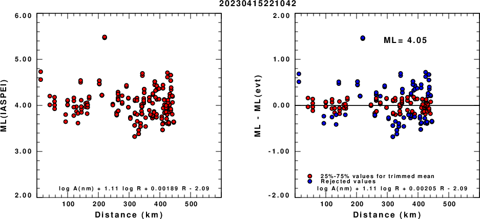
(a) ML computed using the IASPEI formula for Horizontal components; (b) ML residuals computed using a modified IASPEI formula that accounts for path specific attenuation; the values used for the trimmed mean are indicated. The ML relation used for each figure is given at the bottom of each plot.

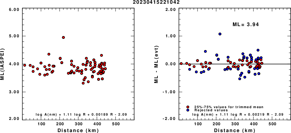
(a) ML computed using the IASPEI formula for Vertical components (research); (b) ML residuals computed using a modified IASPEI formula that accounts for path specific attenuation; the values used for the trimmed mean are indicated. The ML relation used for each figure is given at the bottom of each plot.

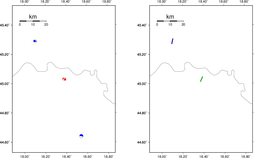
Context

The next figure presents the focal mechanism for this earthquake (red) in the context of other events (blue) in the SLU Moment Tensor Catalog which are within ± 0.5 degrees of the new event. This comparison is shown in the left panel of the figure. The right panel shows the inferred direction of maximum compressive stress and the type of faulting (green is strike-slip, red is normal, blue is thrust; oblique is shown by a combination of colors).

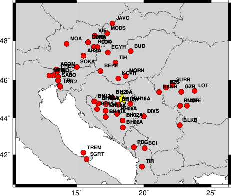
Waveform Inversion using wvfgrd96

The focal mechanism was determined using broadband seismic waveforms. The location of the event and the and stations used for the waveform inversion are shown in the next figure.

Location of broadband stations used for waveform inversion

The program wvfgrd96 was used with good traces observed at short distance to determine the focal mechanism, depth and seismic moment. This technique requires a high quality signal and well determined velocity model for the Green functions. To the extent that these are the quality data, this type of mechanism should be preferred over the radiation pattern technique which requires the separate step of defining the pressure and tension quadrants and the correct strike.

The observed and predicted traces are filtered using the following gsac commands:

cut o DIST/3.3 -40 o DIST/3.3 +50
rtr
taper w 0.1
hp c 0.03 n 3 
lp c 0.10 n 3

The results of this grid search are as follow:

           DEPTH  STK   DIP  RAKE   MW    FIT
WVFGRD96    1.0   240    75   -10   3.46 0.2682
WVFGRD96    2.0   240    60   -15   3.62 0.3404
WVFGRD96    3.0   240    50   -15   3.69 0.3761
WVFGRD96    4.0   245    55     0   3.71 0.4076
WVFGRD96    5.0   245    60     5   3.74 0.4339
WVFGRD96    6.0   250    60    15   3.77 0.4558
WVFGRD96    7.0   250    65    15   3.80 0.4753
WVFGRD96    8.0   250    60    15   3.86 0.4915
WVFGRD96    9.0   250    65    15   3.88 0.4991
WVFGRD96   10.0   250    65    15   3.90 0.5037
WVFGRD96   11.0   250    65    15   3.92 0.5030
WVFGRD96   12.0   250    65    10   3.93 0.4987
WVFGRD96   13.0   250    70    10   3.95 0.4918
WVFGRD96   14.0   250    70    10   3.96 0.4820
WVFGRD96   15.0   250    70    10   3.97 0.4698
WVFGRD96   16.0   250    70     5   3.98 0.4555
WVFGRD96   17.0   250    70     5   3.99 0.4396
WVFGRD96   18.0   250    70     5   4.00 0.4217
WVFGRD96   19.0   250    70     5   4.01 0.4026
WVFGRD96   20.0   250    70     5   4.01 0.3832
WVFGRD96   21.0   250    70     0   4.02 0.3643
WVFGRD96   22.0   250    70     0   4.02 0.3462
WVFGRD96   23.0   250    70     5   4.02 0.3293
WVFGRD96   24.0    70    70    10   4.02 0.3156
WVFGRD96   25.0   160    85   -25   4.02 0.3101
WVFGRD96   26.0   160    85   -25   4.03 0.3086
WVFGRD96   27.0   160    85   -25   4.04 0.3066
WVFGRD96   28.0   160    85   -25   4.04 0.3032
WVFGRD96   29.0   340    90    25   4.05 0.2971

The best solution is

WVFGRD96   10.0   250    65    15   3.90 0.5037

The mechanism correspond to the best fit is

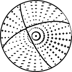
Figure 1. Waveform inversion focal mechanism

The best fit as a function of depth is given in the following figure:

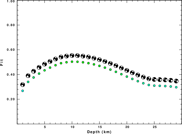
Figure 2. Depth sensitivity for waveform mechanism

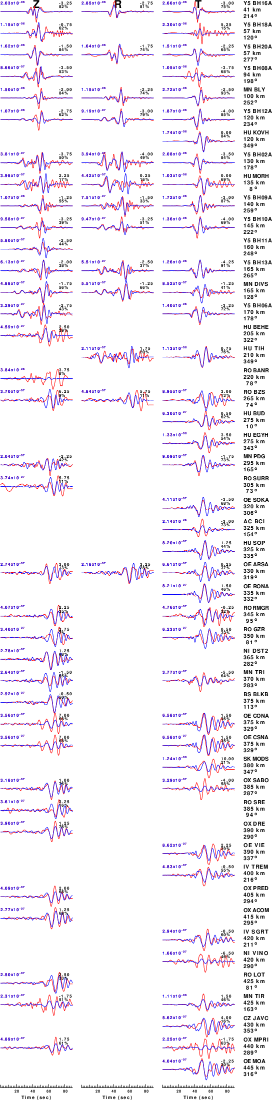
The comparison of the observed and predicted waveforms is given in the next figure. The red traces are the observed and the blue are the predicted. Each observed-predicted component is plotted to the same scale and peak amplitudes are indicated by the numbers to the left of each trace. A pair of numbers is given in black at the right of each predicted traces. The upper number it the time shift required for maximum correlation between the observed and predicted traces. This time shift is required because the synthetics are not computed at exactly the same distance as the observed and because the velocity model used in the predictions may not be perfect. A positive time shift indicates that the prediction is too fast and should be delayed to match the observed trace (shift to the right in this figure). A negative value indicates that the prediction is too slow. The lower number gives the percentage of variance reduction to characterize the individual goodness of fit (100% indicates a perfect fit).

The bandpass filter used in the processing and for the display was

cut o DIST/3.3 -40 o DIST/3.3 +50
rtr
taper w 0.1
hp c 0.03 n 3 
lp c 0.10 n 3

Figure 3. Waveform comparison for selected depth. Red: observed; Blue - predicted. The time shift with respect to the model prediction is indicated. The percent of fit is also indicated. The time scale is based on the last trace plotted. It is not used to represent travel time or absolute time, but rather to indicate the number of seconds plotted. If there is not a trace directly above the scale, then a default, meaningless scale is plotted.

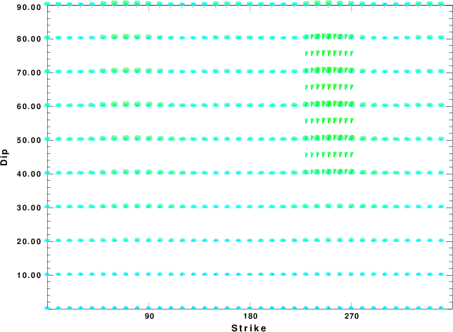
Focal mechanism sensitivity at the preferred depth. The red color indicates a very good fit to thewavefroms. Each solution is plotted as a vector at a given value of strike and dip with the angle of the vector representing the rake angle, measured, with respect to the upward vertical (N) in the figure.

A check on the assumed source location is possible by looking at the time shifts between the observed and predicted traces. The time shifts for waveform matching arise for several reasons:

The origin time and epicentral distance are incorrect
The velocity model used for the inversion is incorrect
The velocity model used to define the P-arrival time is not the same as the velocity model used for the waveform inversion (assuming that the initial trace alignment is based on the P arrival time)

Assuming only a mislocation, the time shifts are fit to a functional form:

 Time_shift = A + B cos Azimuth + C Sin Azimuth

The time shifts for this inversion lead to the next figure:

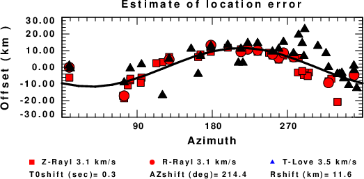
The derived shift in origin time and epicentral coordinates are given at the bottom of the figure.

Discussion

Acknowledgements

Thanks also to the many seismic network operators whose dedication make this effort possible: University of Nevada Reno, University of Alaska, University of Washington, Oregon State University, University of Utah, Montana Bureau of Mines, UC Berkely, Caltech, UC San Diego, Saint Louis University, University of Memphis, Lamont Doherty Earth Observatory, the Oklahoma Geological Survey, TexNet, the Iris stations, the Transportable Array of EarthScope and other networks.

Velocity Model

The WUS.model used for the waveform synthetic seismograms and for the surface wave eigenfunctions and dispersion is as follows:

MODEL.01
Model after     8 iterations
ISOTROPIC
KGS
FLAT EARTH
1-D
CONSTANT VELOCITY
LINE08
LINE09
LINE10
LINE11
      H(KM)   VP(KM/S)   VS(KM/S) RHO(GM/CC)         QP         QS       ETAP       ETAS      FREFP      FREFS
     1.9000     3.4065     2.0089     2.2150  0.302E-02  0.679E-02   0.00       0.00       1.00       1.00    
     6.1000     5.5445     3.2953     2.6089  0.349E-02  0.784E-02   0.00       0.00       1.00       1.00    
    13.0000     6.2708     3.7396     2.7812  0.212E-02  0.476E-02   0.00       0.00       1.00       1.00    
    19.0000     6.4075     3.7680     2.8223  0.111E-02  0.249E-02   0.00       0.00       1.00       1.00    
     0.0000     7.9000     4.6200     3.2760  0.164E-10  0.370E-10   0.00       0.00       1.00       1.00

Quality Control

Here we tabulate the reasons for not using certain digital data sets

The following stations did not have a valid response files:

Last Changed Sat May 6 17:21:31 CDT 2023