Location

Location ANSS

Focal Mechanism

USGS/SLU Moment Tensor Solution ENS 2022/11/09 06:07:27:0 43.93 13.31 10.0 5.8 Marotta, IT Stations used: CH.BERNI CH.DAVOX CH.FIESA CH.FUORN CH.LIENZ CH.VMV CR.STON CR.ZAG GE.MARCO GR.FUR GR.UBR HU.BEHE HU.EGYH HU.KOVH HU.MORH HU.MPLH HU.SOP HU.TIH IV.AOI IV.APEC IV.ARCI IV.ARVD IV.ASSB IV.ATMI IV.ATVO IV.BDI IV.BOSL IV.BRIS IV.BSSO IV.BULG IV.CAFI IV.CAMP IV.CASP IV.CBAC IV.CELB IV.CERT IV.CESI IV.CESX IV.CFMN IV.CING IV.CMPR IV.CMSN IV.CNIS IV.CRE IV.CRMI IV.CRTC IV.CSNT IV.CSOB IV.CTI IV.DGI IV.FAGN IV.FDMO IV.FIAM IV.FIR IV.FNVD IV.FVI IV.GIGS IV.GIUL IV.GUAR IV.GUMA IV.INTR IV.IOCA IV.LATE IV.LMD IV.LNSS IV.LPEL IV.MA9 IV.MCEL IV.MELA IV.MGAB IV.MRLC IV.MSAG IV.MSSA IV.MTCE IV.MTRZ IV.MTSN IV.MURB IV.NARO IV.NRCA IV.OSSC IV.OVO IV.PALZ IV.PAOL IV.PARC IV.PIEI IV.PIGN IV.PII IV.PLMA IV.POFI IV.PSB1 IV.PTCC IV.PTMR IV.PTQR IV.RDP IV.RMP IV.ROSPO IV.SACS IV.SEI IV.SGG IV.SIRI IV.SNTG IV.SORR IV.SRES IV.SSFR IV.STAL IV.T0110 IV.TERO IV.TOLF IV.TREM IV.TRTR IV.VAGA IV.VBKN IV.VCRE IV.VISG IV.VITU IV.VIVA IV.VMGN IV.VTIR IV.VVDG IV.VVLD IV.ZCCA MN.AQU MN.BLY MN.CUC MN.PDG MN.SENA MN.TRI MN.VLC OE.ABTA OE.ARSA OE.BIOA OE.CONA OE.CSNA OE.FETA OE.KBA OE.LESA OE.MOA OE.MOTA OE.MYKA OE.OBKA OE.RETA OE.RONA OE.SOKA OE.SQTA OE.WATA OE.WTTA OX.ACOM OX.AGOR OX.BAD OX.BOO OX.CAE OX.CIMO OX.CLUD OX.FUSE OX.MARN OX.MLN OX.MPRI OX.PLRO OX.PRED OX.SABO OX.VARN SL.BOJS SL.CADS SL.CEY SL.CRES SL.CRNS SL.DOBS SL.GBAS SL.GCIS SL.GOLS SL.GORS SL.GROS SL.JAVS SL.KNDS SL.KOGS SL.LJU SL.MOZS SL.PDKS SL.PERS SL.ROBS SL.SKDS SL.VISS SL.VNDS SL.VOJS SL.ZAVS Filtering commands used: cut o DIST/3.3 -60 o DIST/3.3 +100 rtr taper w 0.1 hp c 0.02 n 3 lp c 0.05 n 3 Best Fitting Double Couple Mo = 2.66e+24 dyne-cm Mw = 5.55 Z = 8 km Plane Strike Dip Rake NP1 290 65 65 NP2 158 35 132 Principal Axes: Axis Value Plunge Azimuth T 2.66e+24 62 161 N 0.00e+00 23 301 P -2.66e+24 16 38 Moment Tensor: (dyne-cm) Component Value Mxx -9.76e+23 Mxy -1.37e+24 Mxz -1.62e+24 Myy -8.71e+23 Myz -8.36e+22 Mzz 1.85e+24 -------------- ##-------------------- ###-------------------- -- ###--------------------- P --- ####---------------------- ----- ####-------------------------------- ####-######--------------------------- ------###############------------------- ------###################--------------- -------#######################------------ -------##########################--------- -------############################------- --------#############################----- -------############## ##############-- --------############# T ###############- --------############ ############### --------############################ ---------######################### --------###################### ----------################## ----------############ -------------- Global CMT Convention Moment Tensor: R T P 1.85e+24 -1.62e+24 8.36e+22 -1.62e+24 -9.76e+23 1.37e+24 8.36e+22 1.37e+24 -8.71e+23 Details of the solution is found at http://www.eas.slu.edu/eqc/eqc_mt/MECH.NA/20221109060727/index.html

Preferred Solution

      STK = 290
      DIP = 65
     RAKE = 65
       MW = 5.55
       HS = 8.0

The NDK file is 20221109060727.ndk The waveform inversion is preferred.

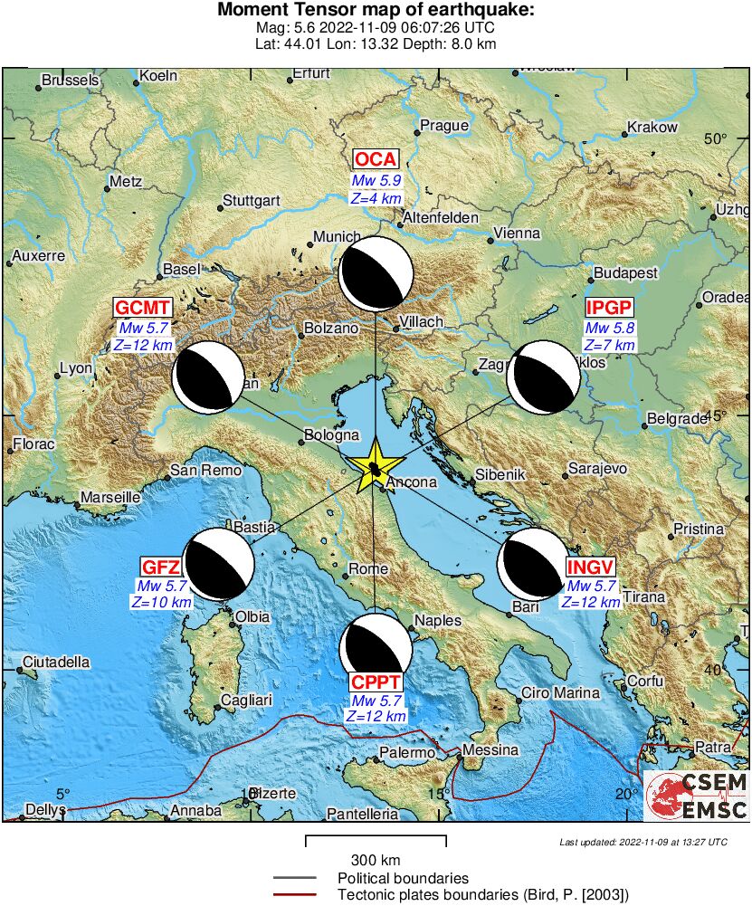
Moment Tensor Comparison

The following compares this source inversion to others

SLU	INGVTDMT	EMSC	SLUCWB
USGS/SLU Moment Tensor Solution ENS 2022/11/09 06:07:27:0 43.93 13.31 10.0 5.8 Marotta, IT Stations used: CH.BERNI CH.DAVOX CH.FIESA CH.FUORN CH.LIENZ CH.VMV CR.STON CR.ZAG GE.MARCO GR.FUR GR.UBR HU.BEHE HU.EGYH HU.KOVH HU.MORH HU.MPLH HU.SOP HU.TIH IV.AOI IV.APEC IV.ARCI IV.ARVD IV.ASSB IV.ATMI IV.ATVO IV.BDI IV.BOSL IV.BRIS IV.BSSO IV.BULG IV.CAFI IV.CAMP IV.CASP IV.CBAC IV.CELB IV.CERT IV.CESI IV.CESX IV.CFMN IV.CING IV.CMPR IV.CMSN IV.CNIS IV.CRE IV.CRMI IV.CRTC IV.CSNT IV.CSOB IV.CTI IV.DGI IV.FAGN IV.FDMO IV.FIAM IV.FIR IV.FNVD IV.FVI IV.GIGS IV.GIUL IV.GUAR IV.GUMA IV.INTR IV.IOCA IV.LATE IV.LMD IV.LNSS IV.LPEL IV.MA9 IV.MCEL IV.MELA IV.MGAB IV.MRLC IV.MSAG IV.MSSA IV.MTCE IV.MTRZ IV.MTSN IV.MURB IV.NARO IV.NRCA IV.OSSC IV.OVO IV.PALZ IV.PAOL IV.PARC IV.PIEI IV.PIGN IV.PII IV.PLMA IV.POFI IV.PSB1 IV.PTCC IV.PTMR IV.PTQR IV.RDP IV.RMP IV.ROSPO IV.SACS IV.SEI IV.SGG IV.SIRI IV.SNTG IV.SORR IV.SRES IV.SSFR IV.STAL IV.T0110 IV.TERO IV.TOLF IV.TREM IV.TRTR IV.VAGA IV.VBKN IV.VCRE IV.VISG IV.VITU IV.VIVA IV.VMGN IV.VTIR IV.VVDG IV.VVLD IV.ZCCA MN.AQU MN.BLY MN.CUC MN.PDG MN.SENA MN.TRI MN.VLC OE.ABTA OE.ARSA OE.BIOA OE.CONA OE.CSNA OE.FETA OE.KBA OE.LESA OE.MOA OE.MOTA OE.MYKA OE.OBKA OE.RETA OE.RONA OE.SOKA OE.SQTA OE.WATA OE.WTTA OX.ACOM OX.AGOR OX.BAD OX.BOO OX.CAE OX.CIMO OX.CLUD OX.FUSE OX.MARN OX.MLN OX.MPRI OX.PLRO OX.PRED OX.SABO OX.VARN SL.BOJS SL.CADS SL.CEY SL.CRES SL.CRNS SL.DOBS SL.GBAS SL.GCIS SL.GOLS SL.GORS SL.GROS SL.JAVS SL.KNDS SL.KOGS SL.LJU SL.MOZS SL.PDKS SL.PERS SL.ROBS SL.SKDS SL.VISS SL.VNDS SL.VOJS SL.ZAVS Filtering commands used: cut o DIST/3.3 -60 o DIST/3.3 +100 rtr taper w 0.1 hp c 0.02 n 3 lp c 0.05 n 3 Best Fitting Double Couple Mo = 2.66e+24 dyne-cm Mw = 5.55 Z = 8 km Plane Strike Dip Rake NP1 290 65 65 NP2 158 35 132 Principal Axes: Axis Value Plunge Azimuth T 2.66e+24 62 161 N 0.00e+00 23 301 P -2.66e+24 16 38 Moment Tensor: (dyne-cm) Component Value Mxx -9.76e+23 Mxy -1.37e+24 Mxz -1.62e+24 Myy -8.71e+23 Myz -8.36e+22 Mzz 1.85e+24 -------------- ##-------------------- ###-------------------- -- ###--------------------- P --- ####---------------------- ----- ####-------------------------------- ####-######--------------------------- ------###############------------------- ------###################--------------- -------#######################------------ -------##########################--------- -------############################------- --------#############################----- -------############## ##############-- --------############# T ###############- --------############ ############### --------############################ ---------######################### --------###################### ----------################## ----------############ -------------- Global CMT Convention Moment Tensor: R T P 1.85e+24 -1.62e+24 8.36e+22 -1.62e+24 -9.76e+23 1.37e+24 8.36e+22 1.37e+24 -8.71e+23 Details of the solution is found at http://www.eas.slu.edu/eqc/eqc_mt/MECH.NA/20221109060727/index.html			USGS/SLU Moment Tensor Solution ENS 2022/11/09 06:07:27:0 43.93 13.31 10.0 5.8 Marotta, IT Stations used: CH.FUORN CZ.KHC G.ECH GE.MATE GE.PSZ GE.STU GR.CLL GR.GRA1 HU.BEHE II.BFO IU.GRFO IV.MURB IV.SGRT MN.AQU MN.BLY MN.BZS MN.CUC MN.DIVS MN.DPC MN.PDG MN.TIP MN.TIR MN.TRI MN.VAE OX.CIMO OX.FUSE OX.PRED OX.SABO Filtering commands used: cut o DIST/3.3 -60 o DIST/3.3 +100 rtr taper w 0.1 hp c 0.02 n 3 lp c 0.05 n 3 Best Fitting Double Couple Mo = 2.75e+24 dyne-cm Mw = 5.56 Z = 8 km Plane Strike Dip Rake NP1 325 60 95 NP2 135 30 81 Principal Axes: Axis Value Plunge Azimuth T 2.75e+24 74 248 N 0.00e+00 4 142 P -2.75e+24 15 51 Moment Tensor: (dyne-cm) Component Value Mxx -9.77e+23 Mxy -1.19e+24 Mxz -6.89e+23 Myy -1.40e+24 Myz -1.19e+24 Mzz 2.38e+24 -------------- ---------------------- #######--------------------- ############--------------- -###############------------- P -- --#################----------- --- --####################---------------- ---######################--------------- ---#######################-------------- ----########################-------------- ----############# #########------------- -----############ T ##########------------ ------########### ###########----------- -----##########################--------- -------########################--------- -------########################------- --------######################------ ---------####################----- ---------##################--- ------------################ ---------------------- -------------- Global CMT Convention Moment Tensor: R T P 2.38e+24 -6.89e+23 1.19e+24 -6.89e+23 -9.77e+23 1.19e+24 1.19e+24 1.19e+24 -1.40e+24 Details of the solution is found at http://www.eas.slu.edu/eqc/eqc_mt/MECH.NA/20221109060727/index.html

Magnitudes

ML Magnitude

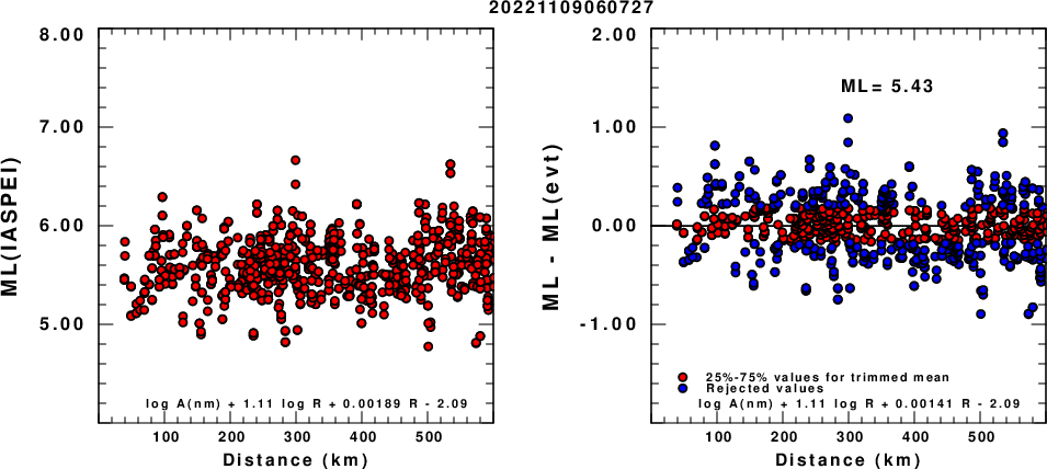
(a) ML computed using the IASPEI formula for Horizontal components; (b) ML residuals computed using a modified IASPEI formula that accounts for path specific attenuation; the values used for the trimmed mean are indicated. The ML relation used for each figure is given at the bottom of each plot.

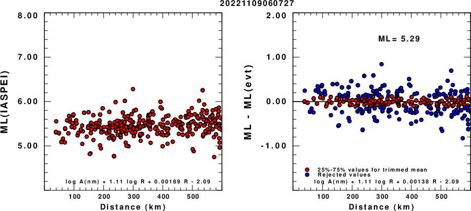
(a) ML computed using the IASPEI formula for Vertical components (research); (b) ML residuals computed using a modified IASPEI formula that accounts for path specific attenuation; the values used for the trimmed mean are indicated. The ML relation used for each figure is given at the bottom of each plot.

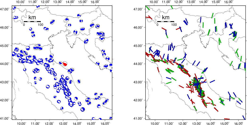
Context

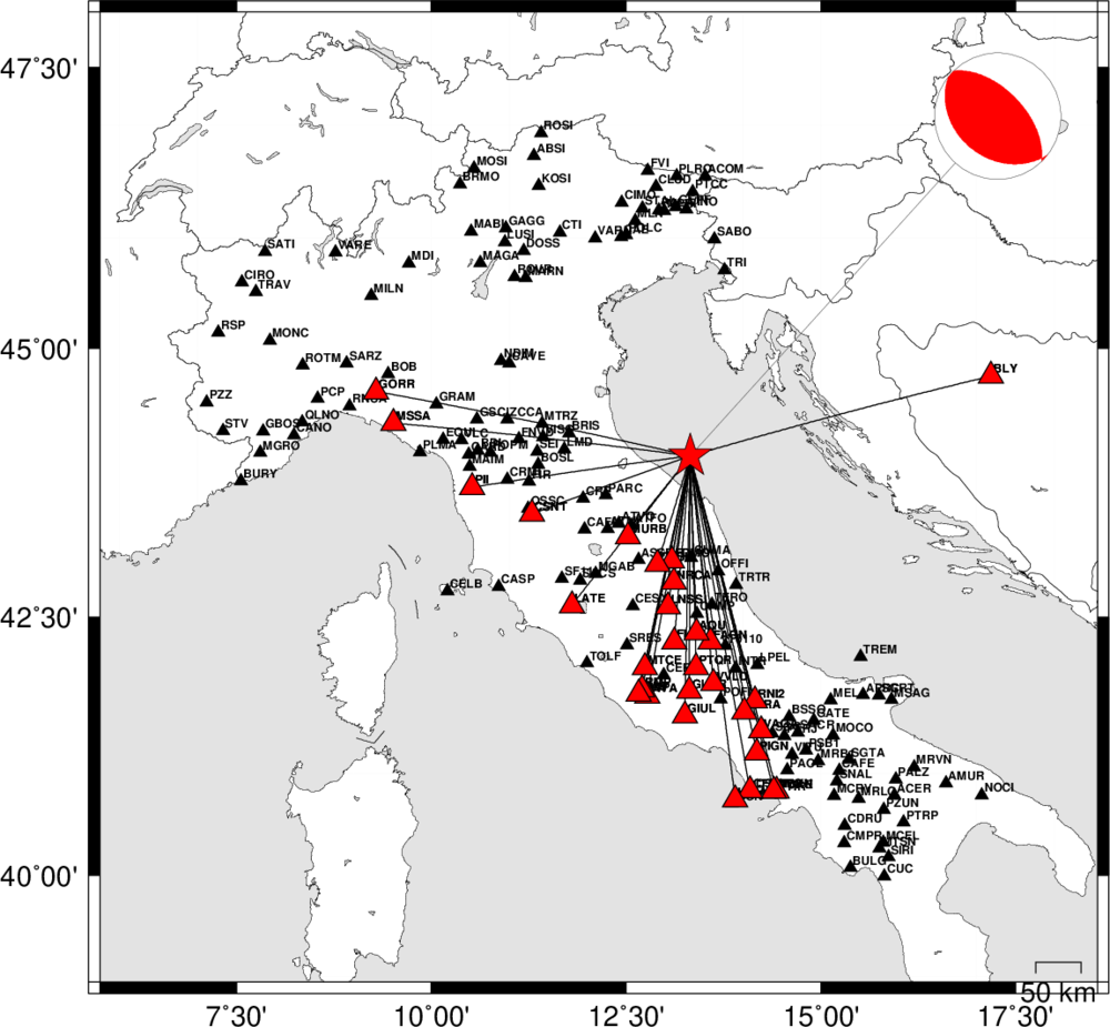
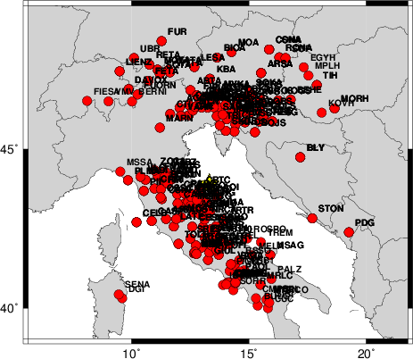
Waveform Inversion

The focal mechanism was determined using broadband seismic waveforms. The location of the event and the and stations used for the waveform inversion are shown in the next figure.

Location of broadband stations used for waveform inversion

The program wvfgrd96 was used with good traces observed at short distance to determine the focal mechanism, depth and seismic moment. This technique requires a high quality signal and well determined velocity model for the Green functions. To the extent that these are the quality data, this type of mechanism should be preferred over the radiation pattern technique which requires the separate step of defining the pressure and tension quadrants and the correct strike.

The observed and predicted traces are filtered using the following gsac commands:

cut o DIST/3.3 -60 o DIST/3.3 +100
rtr
taper w 0.1
hp c 0.02 n 3 
lp c 0.05 n 3 

           DEPTH  STK   DIP  RAKE   MW    FIT
WVFGRD96    1.0   110    45    60   5.28 0.2531
WVFGRD96    2.0   105    45    50   5.37 0.2989
WVFGRD96    3.0   290    60    65   5.43 0.3049
WVFGRD96    4.0   290    65    65   5.47 0.3118
WVFGRD96    5.0   290    65    65   5.48 0.3222
WVFGRD96    6.0   290    65    65   5.49 0.3296
WVFGRD96    7.0   285    65    55   5.49 0.3325
WVFGRD96    8.0   290    65    65   5.55 0.3550
WVFGRD96    9.0   285    65    60   5.54 0.3485
WVFGRD96   10.0   280    70    50   5.52 0.3409
WVFGRD96   11.0   270    85    40   5.51 0.3358
WVFGRD96   12.0    85    85   -30   5.51 0.3345
WVFGRD96   13.0    80    75   -30   5.52 0.3340
WVFGRD96   14.0    80    70   -25   5.52 0.3329
WVFGRD96   15.0    80    70   -25   5.53 0.3318
WVFGRD96   16.0    80    70   -25   5.53 0.3300
WVFGRD96   17.0    80    70   -25   5.54 0.3279
WVFGRD96   18.0    80    70   -25   5.54 0.3255
WVFGRD96   19.0    80    70   -25   5.55 0.3227

The best solution is

WVFGRD96    8.0   290    65    65   5.55 0.3550

The mechanism correspond to the best fit is

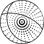
Figure 1. Waveform inversion focal mechanism

The best fit as a function of depth is given in the following figure:

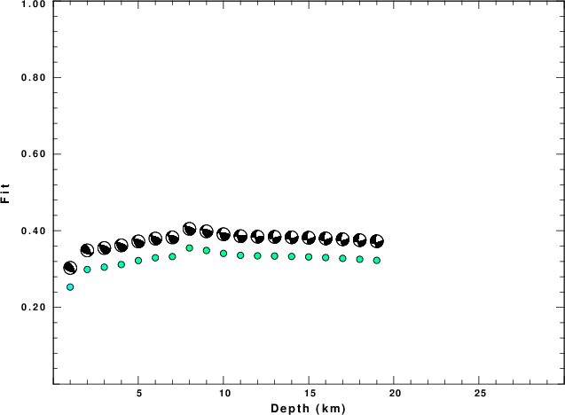
Figure 2. Depth sensitivity for waveform mechanism

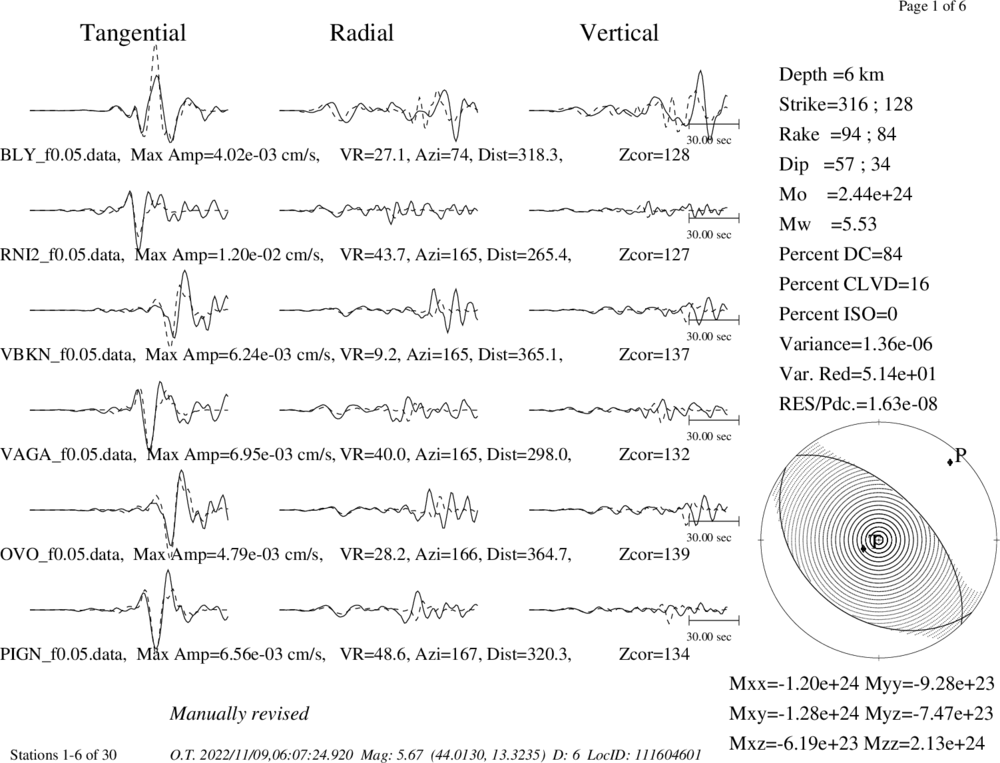
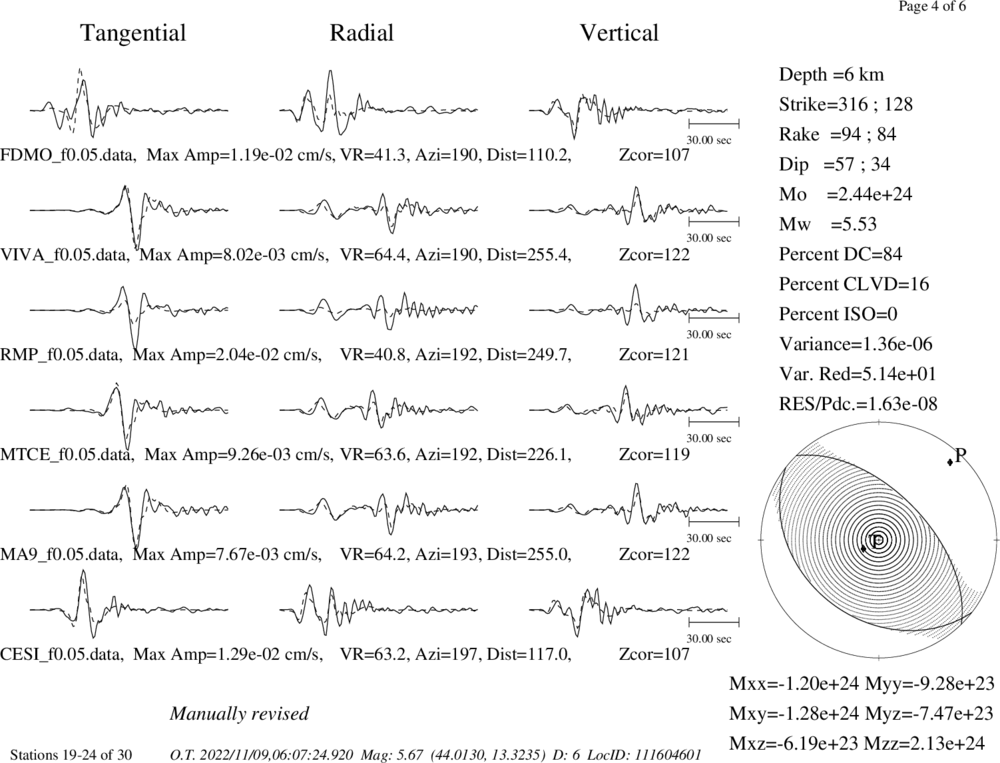
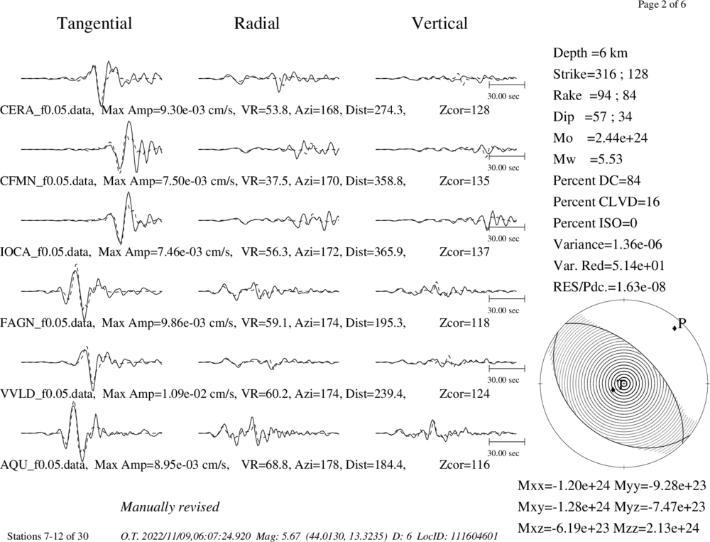
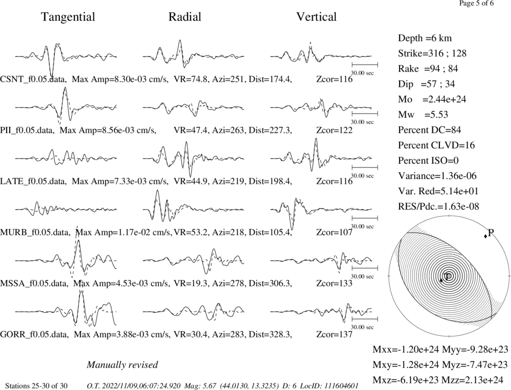
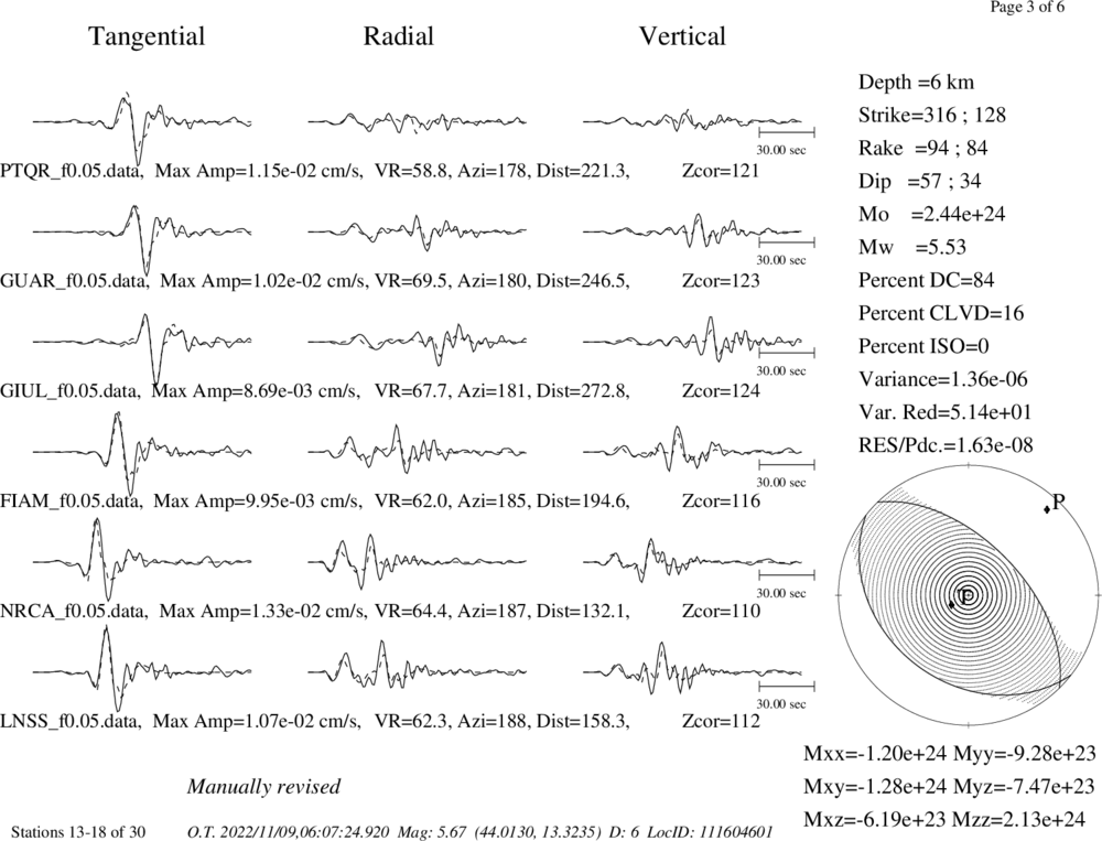
The comparison of the observed and predicted waveforms is given in the next figure. The red traces are the observed and the blue are the predicted. Each observed-predicted component is plotted to the same scale and peak amplitudes are indicated by the numbers to the left of each trace. A pair of numbers is given in black at the right of each predicted traces. The upper number it the time shift required for maximum correlation between the observed and predicted traces. This time shift is required because the synthetics are not computed at exactly the same distance as the observed and because the velocity model used in the predictions may not be perfect. A positive time shift indicates that the prediction is too fast and should be delayed to match the observed trace (shift to the right in this figure). A negative value indicates that the prediction is too slow. The lower number gives the percentage of variance reduction to characterize the individual goodness of fit (100% indicates a perfect fit).

The bandpass filter used in the processing and for the display was

cut o DIST/3.3 -60 o DIST/3.3 +100
rtr
taper w 0.1
hp c 0.02 n 3 
lp c 0.05 n 3 

Figure 3. Waveform comparison for selected depth

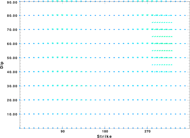
Focal mechanism sensitivity at the preferred depth. The red color indicates a very good fit to thewavefroms. Each solution is plotted as a vector at a given value of strike and dip with the angle of the vector representing the rake angle, measured, with respect to the upward vertical (N) in the figure.

A check on the assumed source location is possible by looking at the time shifts between the observed and predicted traces. The time shifts for waveform matching arise for several reasons:

• The origin time and epicentral distance are incorrect
• The velocity model used for the inversion is incorrect
• The velocity model used to define the P-arrival time is not the same as the velocity model used for the waveform inversion (assuming that the initial trace alignment is based on the P arrival time)

 Time_shift = A + B cos Azimuth + C Sin Azimuth

The time shifts for this inversion lead to the next figure:

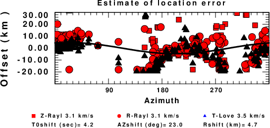
The derived shift in origin time and epicentral coordinates are given at the bottom of the figure.

Discussion

Acknowledgements

Thanks also to the many seismic network operators whose dedication make this effort possible: University of Nevada Reno, University of Alaska, University of Washington, Oregon State University, University of Utah, Montana Bureas of Mines, UC Berkely, Caltech, UC San Diego, Saint Louis University, University of Memphis, Lamont Doherty Earth Observatory, the Iris stations and the Transportable Array of EarthScope.

Velocity Model

The WUS.model used for the waveform synthetic seismograms and for the surface wave eigenfunctions and dispersion is as follows:

MODEL.01
Model after     8 iterations
ISOTROPIC
KGS
FLAT EARTH
1-D
CONSTANT VELOCITY
LINE08
LINE09
LINE10
LINE11
      H(KM)   VP(KM/S)   VS(KM/S) RHO(GM/CC)         QP         QS       ETAP       ETAS      FREFP      FREFS
     1.9000     3.4065     2.0089     2.2150  0.302E-02  0.679E-02   0.00       0.00       1.00       1.00    
     6.1000     5.5445     3.2953     2.6089  0.349E-02  0.784E-02   0.00       0.00       1.00       1.00    
    13.0000     6.2708     3.7396     2.7812  0.212E-02  0.476E-02   0.00       0.00       1.00       1.00    
    19.0000     6.4075     3.7680     2.8223  0.111E-02  0.249E-02   0.00       0.00       1.00       1.00    
     0.0000     7.9000     4.6200     3.2760  0.164E-10  0.370E-10   0.00       0.00       1.00       1.00    

Quality Control

Here we tabulate the reasons for not using certain digital data sets

The following stations did not have a valid response files: