Location

Location SLU

The initial waveform inverion using the EMSC solution required sgnificant time shifts that indicated the need that the epicenter was south of the published solution. First motions and arrival tiems ere read and elocate was use to locate the event using the WUS velocity model. After using the SLU epicenter, the first motions were much better fit by the waveform RMT mechanism. The results of the relocation are given in the file elocate.txt.

The RMT solution is supported by the P-wave first motion. The dip-slip nature of the solution was required by the very low excitation of the Love wave signal on the transverse component.

Location ESMC

Focal Mechanism

USGS/SLU Moment Tensor Solution ENS 2021/08/16 21:15:40:0 47.35 12.07 10.3 4.1 Austria Stations used: BW.ALFT BW.BE1 BW.BGDS BW.BHG BW.BIB BW.FFB1 BW.FFB2 BW.FFB3 BW.GELB BW.KW1 BW.MGBB BW.MGS01 BW.MGS03 BW.MGS05 BW.PART BW.RJOB BW.RMOA BW.RNON BW.ROTZ BW.RTBE BW.RTSA BW.RTSH BW.SCE BW.TON BW.UH3 CH.ACB CH.BERNI CH.BNALP CH.DAVOX CH.EMBD CH.FUORN CH.GRIMS CH.LKBD2 CH.LLS CH.MMK CH.MUGIO CH.PANIX CH.PLONS CH.SIMPL CH.VDR CH.WGT CZ.CKRC CZ.NKC CZ.PRU CZ.STAC CZ.TREC CZ.ZVC GE.STU GR.BFO GR.FUR GR.GEC2 GR.GRA4 GR.GRB1 GR.GRB3 GR.GRB4 GR.GRC1 GR.GRC2 GR.GRC3 GR.GRC4 GR.MILB GR.WET MN.TRI OE.ABTA OE.BIOA OE.CSNA OE.DAVA OE.FETA OE.KBA OE.LESA OE.MOA OE.MYKA OE.SOKA OE.SQTA OE.WATA OX.BAD OX.BALD OX.CAE OX.CLUD OX.FUSE OX.MARN OX.MLN OX.MPRI OX.PRED OX.SABO OX.VARN SX.TANN TH.GRZ1 TH.PLN TH.RANIS TH.ZEU Filtering commands used: cut o DIST/3.3 -30 o DIST/3.3 +70 rtr taper w 0.1 hp c 0.03 n 3 lp c 0.06 n 3 Best Fitting Double Couple Mo = 2.85e+21 dyne-cm Mw = 3.57 Z = 14 km Plane Strike Dip Rake NP1 286 81 102 NP2 50 15 35 Principal Axes: Axis Value Plunge Azimuth T 2.85e+21 52 210 N 0.00e+00 12 104 P -2.85e+21 35 5 Moment Tensor: (dyne-cm) Component Value Mxx -1.08e+21 Mxy 2.98e+20 Mxz -2.53e+21 Myy 2.57e+20 Myz -8.18e+20 Mzz 8.18e+20 -------------- ---------------------- -------------- ----------- --------------- P ------------ ----------------- -------------- ------------------------------------ -------------------------------------# ---------------------------------------# ##########-----------------------------# ###################---------------------## #########################---------------## ###############################---------## ###################################----### ######################################## ############## ####################--- ############# T ###################--- ############ ##################--- ##############################---- ##########################---- -######################----- --##############------ -------------- Global CMT Convention Moment Tensor: R T P 8.18e+20 -2.53e+21 8.18e+20 -2.53e+21 -1.08e+21 -2.98e+20 8.18e+20 -2.98e+20 2.57e+20 Details of the solution is found at http://www.eas.slu.edu/eqc/eqc_mt/MECH.NA/20210816211540/index.html

Preferred Solution

      STK = 50
      DIP = 15
     RAKE = 35
       MW = 3.57
       HS = 14.0

The NDK file is 20210816211540.ndk The waveform inversion is preferred.

Moment Tensor Comparison

The following compares this source inversion to others

SLU

SLUFM

USGS/SLU Moment Tensor Solution ENS 2021/08/16 21:15:40:0 47.35 12.07 10.3 4.1 Austria Stations used: BW.ALFT BW.BE1 BW.BGDS BW.BHG BW.BIB BW.FFB1 BW.FFB2 BW.FFB3 BW.GELB BW.KW1 BW.MGBB BW.MGS01 BW.MGS03 BW.MGS05 BW.PART BW.RJOB BW.RMOA BW.RNON BW.ROTZ BW.RTBE BW.RTSA BW.RTSH BW.SCE BW.TON BW.UH3 CH.ACB CH.BERNI CH.BNALP CH.DAVOX CH.EMBD CH.FUORN CH.GRIMS CH.LKBD2 CH.LLS CH.MMK CH.MUGIO CH.PANIX CH.PLONS CH.SIMPL CH.VDR CH.WGT CZ.CKRC CZ.NKC CZ.PRU CZ.STAC CZ.TREC CZ.ZVC GE.STU GR.BFO GR.FUR GR.GEC2 GR.GRA4 GR.GRB1 GR.GRB3 GR.GRB4 GR.GRC1 GR.GRC2 GR.GRC3 GR.GRC4 GR.MILB GR.WET MN.TRI OE.ABTA OE.BIOA OE.CSNA OE.DAVA OE.FETA OE.KBA OE.LESA OE.MOA OE.MYKA OE.SOKA OE.SQTA OE.WATA OX.BAD OX.BALD OX.CAE OX.CLUD OX.FUSE OX.MARN OX.MLN OX.MPRI OX.PRED OX.SABO OX.VARN SX.TANN TH.GRZ1 TH.PLN TH.RANIS TH.ZEU Filtering commands used: cut o DIST/3.3 -30 o DIST/3.3 +70 rtr taper w 0.1 hp c 0.03 n 3 lp c 0.06 n 3 Best Fitting Double Couple Mo = 2.85e+21 dyne-cm Mw = 3.57 Z = 14 km Plane Strike Dip Rake NP1 286 81 102 NP2 50 15 35 Principal Axes: Axis Value Plunge Azimuth T 2.85e+21 52 210 N 0.00e+00 12 104 P -2.85e+21 35 5 Moment Tensor: (dyne-cm) Component Value Mxx -1.08e+21 Mxy 2.98e+20 Mxz -2.53e+21 Myy 2.57e+20 Myz -8.18e+20 Mzz 8.18e+20 -------------- ---------------------- -------------- ----------- --------------- P ------------ ----------------- -------------- ------------------------------------ -------------------------------------# ---------------------------------------# ##########-----------------------------# ###################---------------------## #########################---------------## ###############################---------## ###################################----### ######################################## ############## ####################--- ############# T ###################--- ############ ##################--- ##############################---- ##########################---- -######################----- --##############------ -------------- Global CMT Convention Moment Tensor: R T P 8.18e+20 -2.53e+21 8.18e+20 -2.53e+21 -1.08e+21 -2.98e+20 8.18e+20 -2.98e+20 2.57e+20 Details of the solution is found at http://www.eas.slu.edu/eqc/eqc_mt/MECH.NA/20210816211540/index.html

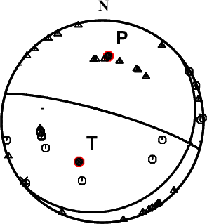
First motions and takeoff angles from an elocate run.

Magnitudes

ML Magnitude

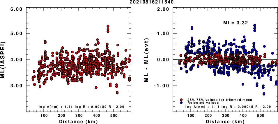
(a) ML computed using the IASPEI formula for Horizontal components; (b) ML residuals computed using a modified IASPEI formula that accounts for path specific attenuation; the values used for the trimmed mean are indicated. The ML relation used for each figure is given at the bottom of each plot.

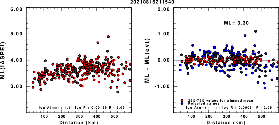
(a) ML computed using the IASPEI formula for Vertical components (research); (b) ML residuals computed using a modified IASPEI formula that accounts for path specific attenuation; the values used for the trimmed mean are indicated. The ML relation used for each figure is given at the bottom of each plot.

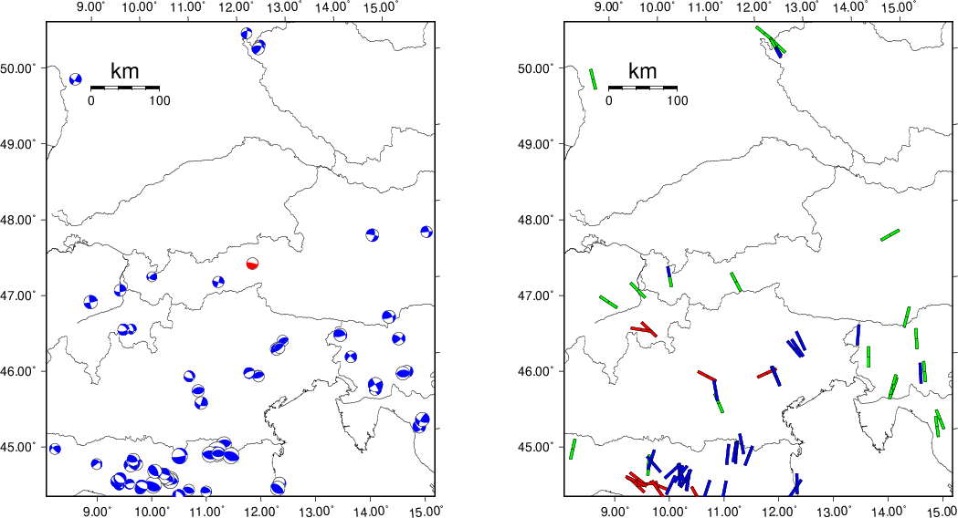
Context

Waveform Inversion

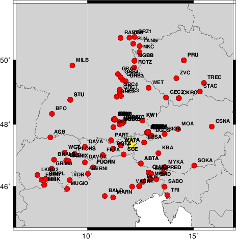
The focal mechanism was determined using broadband seismic waveforms. The location of the event and the and stations used for the waveform inversion are shown in the next figure.

Location of broadband stations used for waveform inversion

The program wvfgrd96 was used with good traces observed at short distance to determine the focal mechanism, depth and seismic moment. This technique requires a high quality signal and well determined velocity model for the Green functions. To the extent that these are the quality data, this type of mechanism should be preferred over the radiation pattern technique which requires the separate step of defining the pressure and tension quadrants and the correct strike.

The observed and predicted traces are filtered using the following gsac commands:

cut o DIST/3.3 -30 o DIST/3.3 +70
rtr
taper w 0.1
hp c 0.03 n 3 
lp c 0.06 n 3 

           DEPTH  STK   DIP  RAKE   MW    FIT
WVFGRD96    1.0   275    45    90   3.31 0.3929
WVFGRD96    2.0    95    45    90   3.41 0.4697
WVFGRD96    3.0   275    30    90   3.45 0.3443
WVFGRD96    4.0    50    20    40   3.48 0.3448
WVFGRD96    5.0    55    15    40   3.49 0.4053
WVFGRD96    6.0    50    15    35   3.49 0.4579
WVFGRD96    7.0    50    15    35   3.48 0.4963
WVFGRD96    8.0    55    15    40   3.56 0.5265
WVFGRD96    9.0    55    15    40   3.56 0.5577
WVFGRD96   10.0    55    15    40   3.56 0.5797
WVFGRD96   11.0    55    15    40   3.56 0.5954
WVFGRD96   12.0    50    15    35   3.56 0.6054
WVFGRD96   13.0    55    15    40   3.57 0.6114
WVFGRD96   14.0    50    15    35   3.57 0.6136
WVFGRD96   15.0    50    15    35   3.57 0.6125
WVFGRD96   16.0    45    15    30   3.58 0.6090
WVFGRD96   17.0   105    75   -85   3.58 0.6040
WVFGRD96   18.0   105    70   -85   3.59 0.6008
WVFGRD96   19.0   105    70   -85   3.59 0.5964
WVFGRD96   20.0   100    65   -80   3.60 0.5905
WVFGRD96   21.0   100    65   -80   3.62 0.5822
WVFGRD96   22.0   105    65   -80   3.62 0.5748
WVFGRD96   23.0   105    65   -80   3.62 0.5666
WVFGRD96   24.0   105    65   -80   3.63 0.5576
WVFGRD96   25.0   105    65   -80   3.63 0.5478
WVFGRD96   26.0   105    65   -80   3.64 0.5374
WVFGRD96   27.0   105    65   -80   3.64 0.5265
WVFGRD96   28.0   105    65   -80   3.65 0.5151
WVFGRD96   29.0   105    65   -80   3.65 0.5032

The best solution is

WVFGRD96   14.0    50    15    35   3.57 0.6136

The mechanism correspond to the best fit is

Figure 1. Waveform inversion focal mechanism

The best fit as a function of depth is given in the following figure:

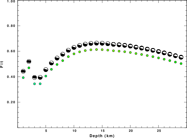
Figure 2. Depth sensitivity for waveform mechanism

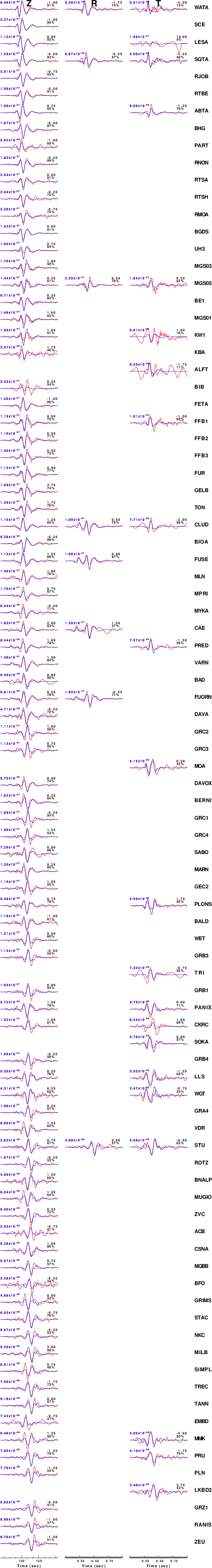
The comparison of the observed and predicted waveforms is given in the next figure. The red traces are the observed and the blue are the predicted. Each observed-predicted component is plotted to the same scale and peak amplitudes are indicated by the numbers to the left of each trace. A pair of numbers is given in black at the right of each predicted traces. The upper number it the time shift required for maximum correlation between the observed and predicted traces. This time shift is required because the synthetics are not computed at exactly the same distance as the observed and because the velocity model used in the predictions may not be perfect. A positive time shift indicates that the prediction is too fast and should be delayed to match the observed trace (shift to the right in this figure). A negative value indicates that the prediction is too slow. The lower number gives the percentage of variance reduction to characterize the individual goodness of fit (100% indicates a perfect fit).

The bandpass filter used in the processing and for the display was

cut o DIST/3.3 -30 o DIST/3.3 +70
rtr
taper w 0.1
hp c 0.03 n 3 
lp c 0.06 n 3 

Figure 3. Waveform comparison for selected depth

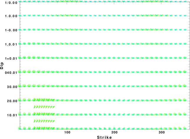
Focal mechanism sensitivity at the preferred depth. The red color indicates a very good fit to thewavefroms. Each solution is plotted as a vector at a given value of strike and dip with the angle of the vector representing the rake angle, measured, with respect to the upward vertical (N) in the figure.

A check on the assumed source location is possible by looking at the time shifts between the observed and predicted traces. The time shifts for waveform matching arise for several reasons:

• The origin time and epicentral distance are incorrect
• The velocity model used for the inversion is incorrect
• The velocity model used to define the P-arrival time is not the same as the velocity model used for the waveform inversion (assuming that the initial trace alignment is based on the P arrival time)

 Time_shift = A + B cos Azimuth + C Sin Azimuth

The time shifts for this inversion lead to the next figure:

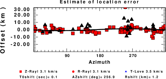
The derived shift in origin time and epicentral coordinates are given at the bottom of the figure.

Discussion

Acknowledgements

Thanks also to the many seismic network operators whose dedication make this effort possible: University of Nevada Reno, University of Alaska, University of Washington, Oregon State University, University of Utah, Montana Bureas of Mines, UC Berkely, Caltech, UC San Diego, Saint Louis University, University of Memphis, Lamont Doherty Earth Observatory, the Iris stations and the Transportable Array of EarthScope.

Velocity Model

The WUS.model used for the waveform synthetic seismograms and for the surface wave eigenfunctions and dispersion is as follows:

MODEL.01
Model after     8 iterations
ISOTROPIC
KGS
FLAT EARTH
1-D
CONSTANT VELOCITY
LINE08
LINE09
LINE10
LINE11
      H(KM)   VP(KM/S)   VS(KM/S) RHO(GM/CC)         QP         QS       ETAP       ETAS      FREFP      FREFS
     1.9000     3.4065     2.0089     2.2150  0.302E-02  0.679E-02   0.00       0.00       1.00       1.00    
     6.1000     5.5445     3.2953     2.6089  0.349E-02  0.784E-02   0.00       0.00       1.00       1.00    
    13.0000     6.2708     3.7396     2.7812  0.212E-02  0.476E-02   0.00       0.00       1.00       1.00    
    19.0000     6.4075     3.7680     2.8223  0.111E-02  0.249E-02   0.00       0.00       1.00       1.00    
     0.0000     7.9000     4.6200     3.2760  0.164E-10  0.370E-10   0.00       0.00       1.00       1.00    

Quality Control

Here we tabulate the reasons for not using certain digital data sets

The following stations did not have a valid response files: